Chapter 8 Other RSM predictions

8.1 TBA How much finished 95%

Work on intro Need better word than constrained finite? discontinuous? end-point-discontinuity?

8.2 TBA Introduction

Chapter 3 described ROC, FROC, AFROC and wAFROC empirical plots and illustrated them using an actual FROC dataset. Chapter 7 described the ROC curve and related quantities predicted by the radiological search model (RSM). This chapter describes the FROC, AFROC and wAFROC curve predictions of the RSM.

Use of a parametric model allows greater insight into the RSM predictions, for example the limiting slopes of the plots at the origin and the end-point, than is possible with empirical plots. Systematic variation of the parameters quantifies some of the expectations based on the solar analogy in Section 2.6. This chapter also illustrates the need for using reasonable values of the parameters - this is achieved using the intrinsic $\lambda_i, \nu_i$ parameters, described in Section 6.6. While the physical parameters $\lambda, \nu$ are easier to understand as relate immediately to the FROC plot end-point, assigning arbitrary values to them can lead to unrealistic predictions.

8.3 RSM-predicted FROC curve

From a property of the Poisson distribution, namely its mean equals the $\lambda$ parameter of the distribution, it follows that the expected number of latent NLs per case is $\lambda$. Recalling that NL z-samples are distributed as N(0,1), one multiplies $\lambda$ by the probability that a z-sample from $N(0,1)$ exceeds $\zeta$, i.e. by $\Phi(-\zeta)$, to obtain the expected number of marked NLs per case, i.e., NLF:

\[\begin{equation} \text{NLF} \left ( \zeta, \lambda \right ) = \lambda \Phi \left (-\zeta \right ) \tag{8.1} \end{equation}\]

We calculate $\text{LLF}$ as follows:

\[\begin{equation} \left. \begin{aligned} \text{LLF} \left ( \mu, \lambda, \nu, \overrightarrow{f_L} \right ) =& \Phi\left ( \mu - \zeta \right )\sum_{L=1}^{L_{max}} f_L \frac{1}{L} \sum_{l_2=0}^{L} \, l_2 \,\, \text{pmf}_{B}\left ( l_2, L, \nu \right )\\ =&\Phi\left ( \mu - \zeta \right )\sum_{L=1}^{L_{max}} f_L \frac{1}{L} L \,\nu\\ =&\nu \,\Phi\left ( \mu - \zeta \right ) \end{aligned} \right \} \tag{8.2} \end{equation}\]

The inner summation is over all cases with $L$ lesions. One calculates the expected value of $l_2$ (the number of lesions that are latent LLs) using the binomial distribution of $l_2$; one divides by $L$ to get the average fraction of LLs on cases with $L$ lesions; one performs an average using the distribution $f_L$ of cases with $L$ lesions; since LL z-samples are distributed as $N(\mu,1)$, one multiplies by the probability that a z-sample from $N(\mu,1)$ exceeds $\zeta$, i.e. by $\Phi(\mu-\zeta)$, to obtain the expected number of marked LLs per case, i.e., LLF. Note that the final expression for LLF is independent of the number of lesions in the dataset or their distribution.

The coordinates of the RSM-predicted operating point on the FROC curve for threshold $\zeta$ are given by Eqn. (8.1) and Eqn. (8.2). The FROC curve starts at (0,0) and ends at $\left ( \lambda, \nu \right )$ – the end-point. The end-point is not constrained to lie within the unit-square, rather it is semi-constrained: while the maximum ordinate, i.e., $\nu$, cannot exceed unity the maximum abscissa, i.e., $\lambda$, can.

The clear connection between $\lambda$ and $\nu$ and the FROC end-point is the reason they are called the physical RSM parameters. For reasons explained in Section 2.6 the physical parameters are not the best way of characterizing predicted RSM curves: they hide an inherent $\mu$ dependence ignoring which can lead to unreasonable choices of RSM parameters (see Appendix 8.7.1). Intrinsic parameters $\lambda_i, \nu_i$ were introduced in Section 6.6 which are independent of $\mu$. For convenience the transformations between physical and intrinsic parameters are reproduced here:

\[\begin{equation} \left. \begin{aligned} \nu =& 1 - \text{exp}\left ( - \mu \nu_i \right ) \\ \lambda =& \frac{\lambda_i}{\mu} \end{aligned} \right \} \tag{8.3} \end{equation}\]

The predicted FROC, AFROC and wAFROC curves that follow use the intrinsic $\lambda_i, \nu_i$ parameters.

8.3.1 FROC plots $\lambda_i, \nu_i$ parameterization

The following code generates FROC plots using the intrinsic $\lambda_i = 2$ and $\nu_i = 0.5$ parameters for 4 values of $\mu$ contained in the array muArr <- c(0.1,1,2,4) (to avoid a divide by zero error the value $\mu=0$ is not allowed). A list array p_FROC_lambdai_nui is created to hold the four plots²⁶. The intrinsic $\lambda_i, \nu_i$ parameters are converted to $\lambda, \nu$ using the function Util2Physical()which implements Eqn. (8.3)). The parameters are displayed using the cat() function. The plots are generated using PlotRsmOperatingCharacteristics(). Online help on this function is available. The code-line p_FROC_lambdai_nui[[i]] <- ret1$FROCPlot saves the plot to the previously created list array.

muArr <- c(0.1,1,2,4)
lambda_i <- 2
nu_i <- 0.5
p_FROC_lambdai_nui <- array(list(), dim = c(length(muArr)))
for (i in 1:length(muArr)) {
  mu <- muArr[i]
  ret <- Util2Physical(mu, lambda_i = lambda_i, nu_i = nu_i)
  lambda <- ret$lambda
  nu <- ret$nu
  cat(sprintf("lambda = %6.3f, nu = %4.3f", lambda, nu), "\n")
  ret1 <- PlotRsmOperatingCharacteristics(
    mu, lambda, nu,
    OpChType = "FROC",
    legendPosition  = "none",
    nlfRange = c(0,4),
    llfRange = c(0,1)
  )
  p_FROC_lambdai_nui[[i]] <- ret1$FROCPlot 
  #+ ggtitle(paste0("mu = ", as.character(muArr[i])))
}

## lambda = 20.000, nu = 0.049 
## lambda =  2.000, nu = 0.393 
## lambda =  1.000, nu = 0.632 
## lambda =  0.500, nu = 0.865

The following code displays the 4 plots.

suppressWarnings(grid.arrange(
p_FROC_lambdai_nui[[1]],
p_FROC_lambdai_nui[[2]],
p_FROC_lambdai_nui[[3]],
p_FROC_lambdai_nui[[4]], ncol = 2))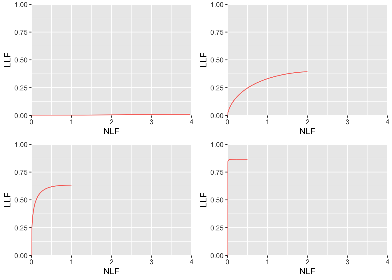

$RSM-predicted FROC curves using intrinsic parameters $\lambda_i = 2$ and $\nu_i = 0.5$. Top left: $\mu = 0.1$; Top right: $\mu = 1$; Bottom left: $\mu = 2$; Bottom right: $\mu = 4$. Some plots are **not** contained within the unit square which makes it impossible to use the FROC-AUC as a figure of merit.$

FIGURE 8.1: RSM-predicted FROC curves using intrinsic parameters $\lambda_i = 2$ and $\nu_i = 0.5$. Top left: $\mu = 0.1$; Top right: $\mu = 1$; Bottom left: $\mu = 2$; Bottom right: $\mu = 4$. Some plots are not contained within the unit square which makes it impossible to use the FROC-AUC as a figure of merit.

In the top-left plot (corresponding to $\mu = 0.1$) because $\lambda = 20$ defines the end-point abscissa and $\nu = 0.049$ defines the end-point ordinate, the FROC curve is close to the x-axis ending at $(20, 0.049)$. For small $\mu$ this is close to the chance line FROC. Recall the solar analogy in Section 2.6. When lesion contrast is low the search mechanism has little chance of finding lesions (leading to small LLF) and generates many NLs in attempting to do so (leading to large NLF).

Increasing $\mu$ to 1 decreases $\lambda$ to 2 and simultaneously increases $\nu$ to 0.393. The new end-point $(2,0.393)$ is evident in the upper-right plot.

Further increase in $\mu$ decreases the abscissa of the end-point and increases the ordinate and the end-point approaches the top-left corner of the FROC plot.

The perfect performance FROC curve is the vertical line connecting the origin to (0,1). It occurs when $\mu = \infty$.

Since the FROC end-point is not constrained to lie within the unit square it is not possible, using the FROC-AUC, to defined a valid figure of merit.

Other characteristics of FROC curves (e.g., slopes at the origin and the end-point) and differences between intrinsic and physical parameterizations of this curve, are explored in Appendix 8.7.1.

8.4 RSM-predicted AFROC curve

The AFROC x-coordinate is the same as the ROC x-coordinate and Eqn. (7.11) applies. The AFROC y-coordinate is identical to the FROC y-coordinate and Eqn. (8.2) applies. Therefore:

\[\begin{equation} \left. \begin{aligned} &\text{FPF}\left (\zeta , \lambda\right ) = 1 - \text{exp}\left ( -\lambda \Phi\left ( -\zeta \right ) \right )\\ &\text{LLF}\left( \zeta, \mu, \nu \right) = \nu \Phi \left ( \mu - \zeta \right ) \end{aligned} \right \} \tag{8.4} \end{equation}\]

The end-point of the AFROC is defined by:

\[\begin{equation} \left. \begin{aligned} \text{FPF}_{\text{max}} =& 1 - \text{exp} \left ( -\lambda \right )\\ \text{LLF}_{\text{max}} =& \nu \end{aligned} \right \} \tag{8.5} \end{equation}\]

Like the ROC the AFROC has the constrained end-point property (i.e., the end-point lies within the unit square) which makes its AUC a valid performance metric.

8.4.1 AFROC plots $\lambda_i, \nu_i$ parameterization

Shown below are AFROC curves for the same parameter values used to demonstrate the preceding FROC curves.

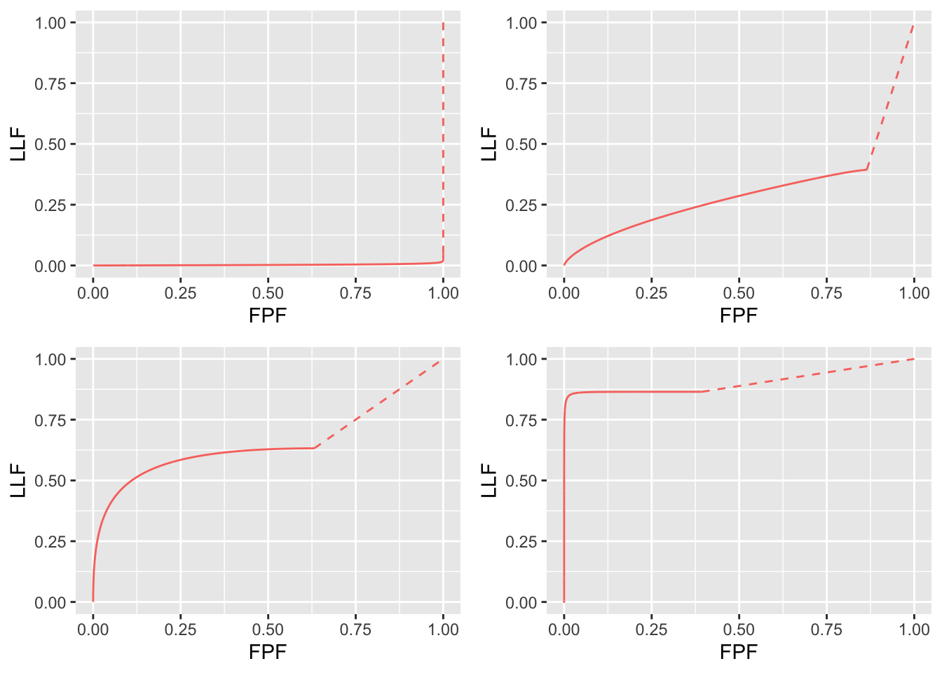
$RSM-predicted AFROC curves using intrinsic parameters $\lambda_i = 2$ and $\nu_i = 0.5$. Top left: $\mu = 0.1$; Top right: $\mu = 1$; Bottom left: $\mu = 2$; Bottom right: $\mu = 4$. Each curve includes an inaccessible dashed linear extension from the end-point to (1,1). Each plot is contained within the unit square and its AUC is a valid figure of merit.$

FIGURE 8.2: RSM-predicted AFROC curves using intrinsic parameters $\lambda_i = 2$ and $\nu_i = 0.5$. Top left: $\mu = 0.1$; Top right: $\mu = 1$; Bottom left: $\mu = 2$; Bottom right: $\mu = 4$. Each curve includes an inaccessible dashed linear extension from the end-point to (1,1). Each plot is contained within the unit square and its AUC is a valid figure of merit.

As discussed in the previous chapter for the ROC, each AFROC curve needs to be completed by a (dashed) straight line extending from the end-point to (1,1). A dashed line is used to distinguish it from the continous curve that is accessible to the observer by appropriate choice of $\zeta$. The inaccessible dashed line is necessary to fully account for all decisions.

Since each plot is contained within the unit square its net (i.e., continuous line plus dashed line) AUC is a valid performance metric.

The AFROC plot is independent of the number of lesions per case. This is not true for the wAFROC, as will shortly become clear, or the ROC (since the ROC ordinate increases with increasing numbers of lesions per case).

As $\mu$ increases the AFROC curve more closely approaches the upper-left corner of the plot and the area under the AFROC curve, including that under the straight line extension, approaches 1, which is the best possible performance.

For $\mu \to 0$ and fixed $\lambda_i$ and $\nu_i$ the operating characteristic approaches the horizontal line extending from the origin to (1,0), which is the continuous section of the curve, followed by the vertical dashed line connecting (1,0) to (1,1) and AFROC-AUC approaches zero. In this limit, no lesion is localized and every case has at least one NL mark, representing worst possible performance.

For $\mu \to \infty$ the accessible portion of the operating characteristic approaches the vertical line connecting (0,0) to (0,1), the area under which is zero. The complete AFROC curve is obtained by connecting this point to (1,1) by the dashed line and in this limit the area under the complete ROC curve approaches 1. As with the ROC, omitting the area under the dashed portion of the curve will result in a severe underestimate of true performance.

Other characteristics of AFROC curves (e.g., slope and differences between intrinsic and physical parameterizations), are explored in Appendix 8.7.3.

8.4.2 Case of the reader who does not make any marks

Suppose the radiologist does not mark any case. One possibility is that the radiologist did not interpret the cases and simply “whizzed” through them. Even though the radiologist is not performing the diagnostic task and the AFROC operating point is stuck at the origin one would still be justified in making the straight-line extension to (1,1) which yields AFROC-AUC = 0.5, which implies finite performance (any value greater than zero for AFROC-AUC implies some degree of expertise). This is because the observer is correct in not marking any non-diseased case (any mark on such a case would be incorrect) and deserves credit for correct decisions on non-diseased cases. The situation is somewhat similar to an ROC study in which all cases are diagnosed as non-diseased - the observer is correct on all non-diseased cases and is rewarded with 100 percent specificity. However, the ROC-AUC for this observer is 0.5 (as the operating point is the origin and one needs to connect it via a dashed straight line to the upper right corner of the ROC plot) and the observer is operating at chance level performance, getting no credit for not marking non-diseased cases.

8.5 RSM-predicted wAFROC curve

The wAFROC abscissa is identical to the ROC abscissa, i.e., Eqn. (7.11) applies. The wAFROC ordinate is calculated using:

\[\begin{equation} \text{wLLF} \left ( \mu, \lambda, \nu, \overrightarrow{f_L}, \mathbf{W} \right ) = \Phi\left ( \mu - \zeta \right )\sum_{L=1}^{L_{max}} f_L \sum_{l_2=1}^{L} \text{W}_{Ll_2} \, l_2 \,\, \text{pmf}_{B}\left ( l_2, L, \nu \right ) \tag{8.6} \end{equation}\]

Note that one does not divide by $L$ outside the inner summation as, for each value of $L$, the weights are already normalized to sum to unit: $\sum_{l_2=1}^{L} \text{W}_{Ll_2}=1$.

Eqn. (8.6) is implemented in UtilAnalyticalAucsRSM. Help is available here. A skeleton code is shown below:

W <-UtilLesWghtsLD(lesDistr, relWeights)
wLLF <- 0
for (L in 1:L_max){
  wLLF_L <- 0
  for (l_2 in 1:L){
    # W has an extra column that must be skipped, hence W[L, l_2+1]
    wLLF_L <- wLLF_L + W[L, l_2+1] * l_2 * dbinom(l_2, L, nu)
  }
  wLLF <- wLLF +  f_L[L] * wLLF_L
}
wLLF <- wLLF * pnorm(mu - zeta)

$\overrightarrow{f_L}$ is the normalized histogram of the lesion distribution for the diseased cases. In the software it is denoted lesDistr. For example, the array lesDistr = c(0.1, 0.4, 0.4, 0.1) defines a dataset in which 10 percent of the cases contain one lesion, 40 percent contain 2 lesions, 40 percent contain 3 lesions and 10 percent contain 4 lesions.
$L_{max}$ is the maximum number of lesions per case in the dataset. In the preceding example $L_{max} = 4$.
$\mathbf{W}$ is the (lower triangular) square weights matrix with $L_{max}$ rows and columns, where each row (excluding cells set to $-\infty$) sums to unity, see example below (the unused matrix elements are set to $-\infty$). In Eqn. (8.6) the index $l_2$ in $W_{Ll_2}$ ranges from 1 to L.
The relative lesion weights are denoted in the code relWeights. For example, relWeights = c(0.2, 0.3, 0.1, 0.5) whose meaning is as follows:
- On cases with one lesion the lesion weight is unity.
- On cases with two lesions the relative weights are 0.2 and 0.3. Since these do not add up to unity, the actual weights are 0.4 and 0.6.
- On cases with three lesions the relative weights are 0.2, 0.3 and 0.1. The actual weights are 1/3, 1/2 and 1/6.
- On cases with four lesions the relative weights are 0.2, 0.3, 0.1 and 0.5. The actual weights are 0.2, 0.3, 0.1 and 0.4.
The function UtilLesWghtsLD calculates the matrix given lesDistr and relWeights. For example:

lesDistr <- c(0.6, 0.2, 0.1, 0.1)
relWeights =  c(0.2, 0.3, 0.1, 0.4)
UtilLesWghtsLD(lesDistr, relWeights)[,-1]

##           [,1] [,2]      [,3] [,4]
## [1,] 1.0000000 -Inf      -Inf -Inf
## [2,] 0.4000000  0.6      -Inf -Inf
## [3,] 0.3333333  0.5 0.1666667 -Inf
## [4,] 0.2000000  0.3 0.1000000  0.4

It is necessary to label the lesions properly so that the correct weights are used. This is done using the lesionID field in the Excel input file. For example, lesionID = 3 for the one with relative weight 0.1. Since $\mathbf{W}$ is independent of cases, the lesion characteristics (which determine outcome/importance) of the lesion with lesionID = 1 in cases with one lesion or in cases with 4 lesions are identical. In other words this example assumes that the lesions fall into four classes, with clinical outcomes as specified in relWeights.
$\text{pmf}_{B}\left ( l_2, L, \nu \right )$ is the probability mass function (pmf) of the binomial distribution with success probability $\nu$ and trial size $L$. $\text{W}_{Ll_2}$ is the weight of lesion $l_2$ in cases with $L$ lesions; for example $\text{W}_{42} = 0.3$.
To generate equal weights set relWeights = 0 as in following code:

lesDistr <- c(0.6, 0.2, 0.1, 0.1)
relWeights0 <- 0
UtilLesWghtsLD(lesDistr, relWeights = relWeights0)[,-1]

##           [,1]      [,2]      [,3] [,4]
## [1,] 1.0000000      -Inf      -Inf -Inf
## [2,] 0.5000000 0.5000000      -Inf -Inf
## [3,] 0.3333333 0.3333333 0.3333333 -Inf
## [4,] 0.2500000 0.2500000 0.2500000 0.25

8.5.1 wAFROC plots $\lambda_i, \nu_i$ parameterization

Shown below are wAFROC curves for the same parameter values used to display the AFROC curves shown in Fig. 8.5.

Note that it is necessary to specify lesDistr when requesting a wAFROC plot. A dataset with a maximum of 4 lesions per diseased case is assumed, with lesDistr <- c(0.6, 0.2, 0.1, 0.1).

p_wAFROC_lambdai_nui <- array(list(), dim = c(length(muArr)))
for (i in 1:length(muArr)) {
  mu <- muArr[i]
  ret <- Util2Physical(mu, lambda_i = lambda_i, nu_i = nu_i)
  lambda <- ret$lambda  
  nu <- ret$nu
  ret1 <- PlotRsmOperatingCharacteristics(
    mu, lambda, nu,
    lesDistr = lesDistr,
    relWeights = relWeights,
    OpChType = "wAFROC",
    legendPosition  = "none"
  )
  p_wAFROC_lambdai_nui[[i]] <- ret1$wAFROCPlot 
  #+ ggtitle(paste0("mu = ", as.character(muArr[i]), 
  #+ ", AUC = ", format(ret1$aucAFROC, digits = 3)))
}

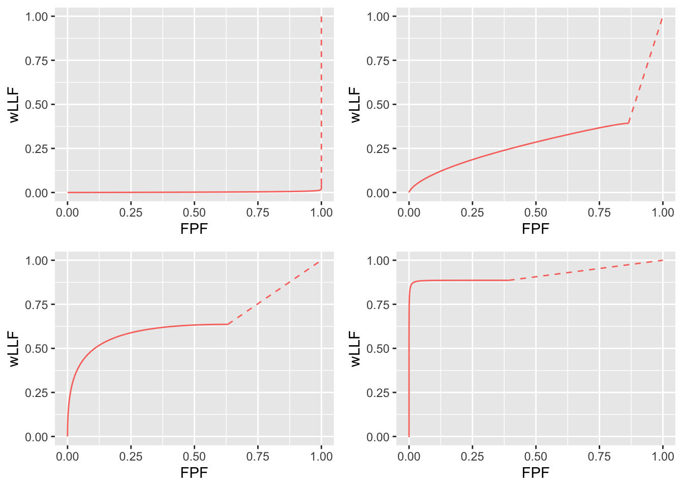
$RSM-predicted wAFROC curves using intrinsic parameters $\lambda_i = 2$ and $\nu_i = 0.5$. Top left: $\mu = 0.1$. Top right: $\mu = 1$. Bottom left: $\mu = 2$. Bottom right: $\mu = 4$. As $\mu$ increases the curve approaches the top-left corner. Each curve includes an inaccessible dashed linear extension to (1,1). Since the plot is contained within the unit square its AUC is a valid figure of merit.$

FIGURE 8.3: RSM-predicted wAFROC curves using intrinsic parameters $\lambda_i = 2$ and $\nu_i = 0.5$. Top left: $\mu = 0.1$. Top right: $\mu = 1$. Bottom left: $\mu = 2$. Bottom right: $\mu = 4$. As $\mu$ increases the curve approaches the top-left corner. Each curve includes an inaccessible dashed linear extension to (1,1). Since the plot is contained within the unit square its AUC is a valid figure of merit.

8.6 Comments on end-point-discontinuity property

RSM predicted ROC, AFROC and wAFROC curves share the end-point-discontinuity property (not extending continuously to (1,1)) that makes them qualitatively different from predictions of all other observer performance models that I am aware of. In my experience this is a property that most researchers in this field have difficulty with. There is simply too much history going back to the early 1940s of the ROC curve extending continuously from (0,0) to (1,1).

I am not aware of any empirical evidence that observers can actually operate continuously in the range (0,0) to (1,1) in search tasks, so the existence of such an ROC is an assumption. In contrast the ROC of an (algorithmic) observer in a non-search task can extend continuously to (1,1). Consider a diagnostic test that rates the results of a laboratory measurement, e.g., the A1C measure of blood glucose for presence of a disease. If $A1C \ge 0.065$ the patient is diagnosed as diabetic. By moving the threshold from $+\infty$ to $-\infty$, and assuming a large population of patients, one can trace out the entire ROC curve from the origin to (1,1). This is because every patient yields an A1C value. Now imagine that some finite fraction of the test results are “lost in the mail”; then the ROC curve, calculated over all patients, will have the end-point-discontinuity property, albeit due to an unreasonable cause.

The situation in medical imaging involving search tasks is more realistic. Not every case yields a decision variable. There is a reasonable cause for this – to render a decision variable sample the radiologist must find something suspicious to report, and if none is found, there is no decision variable to report. The ROC curve calculated over all patients would exhibit the end-point-discontinuity property, even in the limit of an infinite number of patients. If calculated over only those patients that yielded at least one mark, the ROC curve would extend from (0,0) to (1,1) but then one would be ignoring all cases with no marks. For non-diseased cases these represent correct decisions and for diseased cases they represent incorrect decisions and ignoring all cases with no marks should raise concern regarding validity of the analysis.

8.7 Appendix

Unlike the previous plots which used the intrinsic parameters $\lambda_i, \nu_i$, the plots shown here are for arbitrary choices of RSM physical parameters $\lambda, \nu$. This can lead to peculiar predictions arising from physically unreasonable parameter values.

8.7.1 Slope of the FROC curve

Expressions for LLF and NLF were given above. Taking the derivatives of these functions with respect to $\zeta$ the slope of the FROC is given by:

With some simplification this yields:

\[\begin{equation} \left. \begin{aligned} \frac{\frac{\partial }{\partial \zeta}\left( LLF \right)}{\frac{\partial }{\partial \zeta}\left( NLF \right)} =& \frac{\nu}{\lambda} \frac{\text{exp}\left ( \frac{-\left (\mu-\zeta \right )^2}{2} \right )}{\text{exp}\left ( \frac{-\zeta^2}{2} \right )} \\ =& \frac{\nu}{\lambda} \text{exp}\left (-\frac{1}{2} \left( \mu^2 - 2\mu\zeta \right)\right ) \\ \end{aligned} \right \} \tag{8.8} \end{equation}\]

Converting to intrinsic parameters leads to the following expression for the slope:

\[\begin{equation} \left. \begin{aligned} \frac{\frac{\partial }{\partial \zeta}\left( LLF \right)}{\frac{\partial }{\partial \zeta}\left( NLF \right)} =& \mu \left( \frac{1 - \text{exp}\left ( - \mu \nu_i \right ) }{\lambda_i} \right) \text{exp}\left (-\frac{1}{2} \left( \mu^2 - 2\mu\zeta \right) \right ) \end{aligned} \right \} \tag{8.9} \end{equation}\]

Eqn. (8.9) leads to the following conclusions (recall $\mu \ge 0$):

The slope of the FROC near the end-point, corresponding to $\zeta = -\infty$, is zero.

The slope near the origin, corresponding to $\zeta = +\infty$, is $\infty$ provided $\mu \ne 0$.

For $\mu = 0$ the slope of the FROC is zero regardless of the value of $\zeta$, see top-left panel in Fig. 8.1.

If instead we had used Eqn. (8.8) the last conclusion would change to:

For $\mu = 0$ the FROC is predicted to be a straight line extending from the origin to $(\lambda, \nu)$, as in the top-left plot in Fig. 8.4 corresponding to $\mu=0$, $\lambda = 1$ and $\nu = 0.2$. This is unreasonable since for zero contrast lesions the observer should not be able to localize any lesions at finite NLF. The unreasonable prediction is occurring because one is using unrealistic values for the RSM parameters. For zero $\mu$ one expects $\lambda = \infty$ and $\nu = 0$, not $\lambda = 1$ and $\nu = 0.2$.

8.7.2 FROC plots $\lambda, \nu$ parameterization

FROC plots are shown below illustrating the statements just made.

## mu =  0.100, lambda =  1.000, nu = 0.200 
## mu =  1.000, lambda =  2.000, nu = 0.500 
## mu =  2.000, lambda =  3.000, nu = 0.700 
## mu =  4.000, lambda =  4.000, nu = 0.900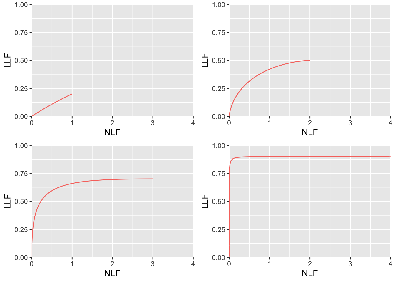

$RSM-predicted FROC curves using $\lambda, \nu$ paramterization. Top left: $\mu = 0.1$, $\lambda = 1$ and $\nu = 0.2$. Top right: $\mu = 1$, $\lambda = 2$ and $\nu = 0.5$. Bottom left: $\mu = 2$, $\lambda = 3$ and $\nu = 0.7$. Bottom right: $\mu = 4$, $\lambda = 4$ and $\nu = 0.9$. The top-left panel is an unrealistic prediction because of unrealistic parameters $\lambda =1, \nu = 0.2$ for small $\mu$.$

FIGURE 8.4: RSM-predicted FROC curves using $\lambda, \nu$ paramterization. Top left: $\mu = 0.1$, $\lambda = 1$ and $\nu = 0.2$. Top right: $\mu = 1$, $\lambda = 2$ and $\nu = 0.5$. Bottom left: $\mu = 2$, $\lambda = 3$ and $\nu = 0.7$. Bottom right: $\mu = 4$, $\lambda = 4$ and $\nu = 0.9$. The top-left panel is an unrealistic prediction because of unrealistic parameters $\lambda =1, \nu = 0.2$ for small $\mu$.

8.7.3 Slope of the AFROC curve

The AFROC ordinate is LLF and the abscissa is FPF. Expressions for both were given above. Taking the derivatives of these functions with respect to $\zeta$ the slope of the continuous section of the AFROC is given by:

\[\begin{equation} \left. \begin{aligned} \frac{\frac{\partial }{\partial \zeta}\left( LLF \right)}{\frac{\partial }{\partial \zeta}\left( FPF \right)} =& \frac{\nu \phi \left ( \mu-\zeta \right )}{\text{exp}\left( -\lambda \Phi\left(- \zeta \right)\left( \lambda\phi\left( -\zeta \right) \right) \right)} \end{aligned} \right \} \tag{8.10} \end{equation}\]

Using Eqn. (8.7) the slope of the AFROC can be expressed in terms of the slope of the FROC:

\[\begin{equation} \left. \begin{aligned} \frac{\frac{\partial }{\partial \zeta}\left( LLF \right)}{\frac{\partial }{\partial \zeta}\left( FPF \right)} =& \frac{\frac{\frac{\partial }{\partial \zeta}\left( LLF \right)}{\frac{\partial }{\partial \zeta}\left( NLF \right)}}{\text{exp}\left ( -\lambda \Phi\left ( -\zeta \right ) \right )}\\ =& \frac{\frac{\frac{\partial }{\partial \zeta}\left( LLF \right)}{\frac{\partial }{\partial \zeta}\left( NLF \right)}}{1-FPF\left( \lambda, \zeta \right)}\\ \end{aligned} \right \} \tag{8.11} \end{equation}\]

The numerator is the slope of the FROC. Since $0 \le \text{FPF} \le \text{FPF}_{\text{max}}$ and $\text{FPF}$ increases as $\zeta$ decreases, the slope of the AFROC equals that of the FROC at the origin and subsequently increases over that of the FROC as the end-point is approached.

This expression leads to the following conclusions, if using intrinsic parameterization:

The slope of the AFROC near the end-point, corresponding to $\zeta = -\infty$, is zero provided $\mu \ne 0$.

The slope near the origin, corresponding to $\zeta = +\infty$, is $\infty$ provided $\mu \ne 0$.

For $\mu = 0$ the slope of the AFROC is zero regardless of the value of $\zeta$, see top-left panel in Fig. 8.2.

If using physical parameters the last conclusion changes to:

For $\mu = 0$ the slope of the AFROC curve increases as the end-point is approached, i.e., the FROC curve is concave up, see top-left panel in Fig. 8.5. The unreasonable prediction is due to the unreasonable choice of parameters.

## mu =  0.100, lambda =  1.000, nu = 0.200 
## mu =  1.000, lambda =  2.000, nu = 0.500 
## mu =  2.000, lambda =  3.000, nu = 0.700 
## mu =  4.000, lambda =  4.000, nu = 0.900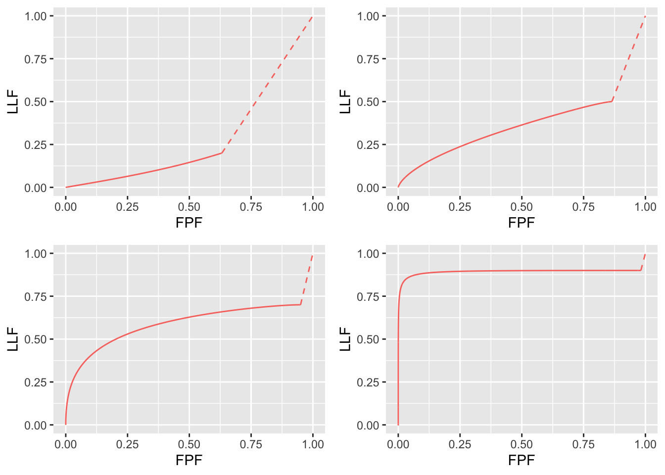

$RSM-predicted AFROC curves, $\lambda, \nu$ paramterization, using same parameter choices as in preceding plot. Note the unrealistic concave up feature of the top-left plot due to unrealistic choices of parameters.$

FIGURE 8.5: RSM-predicted AFROC curves, $\lambda, \nu$ paramterization, using same parameter choices as in preceding plot. Note the unrealistic concave up feature of the top-left plot due to unrealistic choices of parameters.

8.7.4 wAFROC plots $\lambda, \nu$ parameterization

## mu =  0.100, lambda =  1.000, nu = 0.200 
## mu =  1.000, lambda =  2.000, nu = 0.500 
## mu =  2.000, lambda =  3.000, nu = 0.700 
## mu =  4.000, lambda =  4.000, nu = 0.900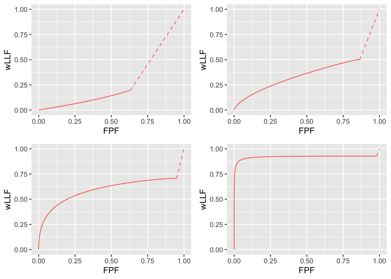

$RSM-predicted wAFROC curves, $\lambda, \nu$ paramterization, using same parameter choices as in preceding plot. Note the unrealistic concave up feature of the top-left plot due to unrealistic choices of parameters.$

FIGURE 8.6: RSM-predicted wAFROC curves, $\lambda, \nu$ paramterization, using same parameter choices as in preceding plot. Note the unrealistic concave up feature of the top-left plot due to unrealistic choices of parameters.

8.7.5 ROC curves are above AFROC curves

Since they share a common x-axis one can compare the relative position of ROC and AFROC curves for the same parameter values, i.e., does one lie above or below the other. Using previous equations for the ROC-TPF and the AFROC-LLF, and focusing on cases with $L$ lesions, one has:

\[\begin{equation} \left. \begin{aligned} & \text{TPF}-\text{LLF} \\ &= 1 - \text{exp}\left ( - \lambda \Phi \left ( - \zeta \right )\right ) \left ( 1 - \nu \Phi \left ( \mu - \zeta \right ) \right )^L - \nu \Phi \left ( \mu - \zeta \right )\\ &= 1 - \nu \Phi \left ( \mu - \zeta \right )- \text{exp}\left ( - \lambda \Phi \left ( - \zeta \right )\right ) \left ( 1 - \nu \Phi \left ( \mu - \zeta \right ) \right )^L \\ &= \left( 1 - \nu \Phi \left ( \mu - \zeta \right ) \right)\left[ 1 - \text{exp}\left ( - \lambda \Phi \left ( - \zeta \right )\right ) \left ( 1 - \nu \Phi \left ( \mu - \zeta \right ) \right )^{L-1} \right]\\ & \ge0 \end{aligned} \right \} \tag{8.12} \end{equation}\]

The final inequality follows from the facts that:

$1 - \nu \Phi \left ( \mu - \zeta \right )$ is non-negative and less than or equal to one, and so are any integer powers of this quantity.
$\text{exp}\left ( - \lambda \Phi \left ( - \zeta \right )\right )$ is non-negative and less than or equal to one.
The equality is achieved when $\zeta = +\infty$, i.e., at the origin (since the $\Phi$ function evaluates to zero).
Averaging over $f_L$, the distribution of lesions, does not change the final conclusion.

The basic reason why TPF is greater than LLF is that the ROC gives credit for incorrect localizations on diseased cases while the AFROC does not. This is the well-known “right for wrong reason” argument (Bunch et al. 1977), originally advanced in 1977, against usage of the ROC for localization tasks.

8.7.6 Are wAFROC curves above AFROC curves?

The following expression follows for the difference between wLLF and LLF:

\[\begin{equation} \left. \begin{aligned} \text{wLLF}-\text{LLF} = \Phi\left ( \mu - \zeta \right )\sum_{L=1}^{L_{max}} f_L \sum_{l_2=1}^{L} \left( \text{W}_{Ll_2} -\frac{1}{L} \right) \, l_2 \,\, \text{pmf}_{B}\left ( l_2, L, \nu \right ) \end{aligned} \right \} \tag{8.13} \end{equation}\]

Since for equally weighted lesions each lesion weight is $\frac{1}{L}$, this equation shows immediately that for equally weighted lesions the difference is zero, i.e., for equally weighted lesions the wAFROC and the AFROC are identical:

\[\begin{equation} \left| \text{wLLF} \right|_\text{equal weights} -\text{LLF} = 0 \tag{8.14} \end{equation}\]

In the general case the two curves are not identical although, for realistic datasets, the differences tend to be small. For cases with L lesions the probability mass function of the binomial distribution is peaked near $l_2 =L\nu$. If the weights array $W_{Ll_2}$ is likewise peaked near $l_2 =L\nu$ the difference tends to be positive, i.e., the wAFROC is above the AFROC. Otherwise the difference can be negative.

REFERENCES

Bunch, Philip C, John F Hamilton, Gary K Sanderson, and Arthur H Simmons. 1977. “A Free Response Approach to the Measurement and Characterization of Radiographic Observer Performance.” In Application of Optical Instrumentation in Medicine VI, 127:124–35. International Society for Optics; Photonics.

Notation: p_ stands for a plot array, FROC stands for type of plot (also allowed are AFROC and wAFROC), lambdai stands for $\lambda_i$ and nui stands for $\nu_i$ (also allowed are lambda for $\lambda$ and nu for $\nu$ ).↩︎

The RJafroc Froc Book