Chapter 3 Modeling the binary Task
3.2 Introduction
Chapter 3 introduced measures of performance associated with the binary task. Described in this chapter is a 2-parameter statistical model for the binary task. It shows how one can predict quantities like sensitivity and specificity based on the values of the parameters of a statistical model of the binary task. Introduced are the fundamental concepts of a decision variable and a reporting threshold or simple threshold that occur frequently in this book. It is shown that the reporting threshold can be altered by varying the experimental conditions. The receiver-operating characteristic (ROC) plot is introduced. It is shown how the dependence of sensitivity and specificity on the reporting threshold can be exploited by a measure of performance that is independent of reporting threshold.
The dependence of variability of the operating point on the numbers of cases is examined. The concept of random sampling is introduced and it is shown that the results become more stable with larger numbers of cases, i.e., larger sample sizes. These are perhaps intuitively obvious concepts but it is important to see them demonstrated, Online Appendix 3.A. Formulae for confidence intervals for estimates of sensitivity and specificity are derived and the calculations are shown explicitly using R code.
3.3 Decision variable and reporting threshold
The model for the binary task involves three assumptions:
Each case has an associated decision variable sample.
The observer (e.g., radiologist) adopts a case-independent reporting threshold.
An adequate number of training session(s) are used to get the observer to a steady state.
The observer is “blinded” to the truth of each case while the researcher is not.
3.3.1 Existence of a decision variable
Assumption 1: Each case presentation is associated with the occurrence (or realization) of a value of a random scalar sensory variable which is a unidirectional measure of evidence of disease.
The sensory variable is sensed internally by the observer and as such cannot be directly measured. Alternative terminology includes “psychophysical variable”, “perceived variable”, “perceptual variable” or “confidence level”. The last term is the most common. It is a subjective variable since it depends on the observer: the same case shown to different observers could evoke different values of the sensory variable. Since one cannot measure it anyway, it would be a very strong assumption to assume that the sensations are identical. In this book the term “latent decision variable” or simply “decision variable” is used, which hopefully gets away from the semantics and focuses instead on what the variable is used for, namely making decisions. The symbol \(Z\) is used and specific realized values are termed z-samples. It is a random variable in the sense that it varies randomly from case to case.
The decision variable rank-orders cases with respect to evidence for presence of disease. Unlike a traditional rank-ordering scheme, where “1” is the highest rank, the scale is inverted with larger values corresponding to greater evidence of disease. Without loss of generality, one assumes that the decision variable ranges from \(-\infty\) to \(+\infty\) with large positive values indicative of strong evidence for presence of disease and large negative values indicative of strong evidence for absence of disease. The zero value indicates no evidence for presence or absence of disease. 2 In this book such a decision scale, with increasing values corresponding to increasing evidence of disease, is termed positive-directed.
3.3.2 Existence of a reporting threshold
Assumption 2: The radiologist adopts a single case-independent reporting threshold \(\zeta\) and states: “case is diseased” if \(z \ge \zeta\) or “case is non-diseased” if \(z < \zeta\).
Unlike the random Z-sample, which varies from case to case, the reporting threshold is held fixed for the duration of the study. In some of the older literature the reporting threshold is sometimes referred to as “response bias”. The term “bias” which has a negative connotation, whereas, in fact, the choice of reporting threshold depends on a rational assessment of costs and benefits of different outcomes.
The choice of reporting threshold depends on the conditions of the study: perceived or known disease prevalence, cost-benefit considerations, instructions regarding dataset characteristics, personal interpreting style, etc. There is a transient “learning curve” during which observer is assumed to find the optimal threshold and henceforth holds it constant for the duration of the study. The learning is expected to stabilize after a sufficiently long training interval.
Data should only be collected in the fixed threshold state, i.e., at the end of the training session.
If a second study is conducted under different conditions, the observer is assumed to determine after a new training session the optimal threshold for the new conditions and henceforth holds it constant for the duration of the second study.
From Assumption 2, it follows that:
\[\begin{equation} \text{1-Sp} \equiv \text{FPF}=P(Z\ge \zeta|T=1) \tag{3.1} \end{equation}\]
\[\begin{equation} \text{Se} \equiv \text{TPF}=P(Z\ge \zeta|T=2) \tag{3.2} \end{equation}\]
Explanation: \(P(Z\ge \zeta|T=1)\) is the probability that the Z-sample for a non-diseased case is greater than or equal to \(\zeta\). According to Assumption 2 these cases are incorrectly classified as diseased, i.e., they are FP decisions, therefore the corresponding probability is false positive fraction \(\text{FPF}\), which is the complement of specificity \(\text{Sp}\). Likewise, \(P(Z\ge \zeta|T=2)\) denotes the probability that the Z-sample for a diseased case is greater than or equal to \(\zeta\). These cases are correctly classified as diseased, i.e., these are TP decisions and the corresponding probability is true positive fraction \(\text{TPF}\), which is sensitivity \(\text{Se}\).
There are several concepts implicit in Eqn. (3.1) and Eqn. (3.2).
The Z-samples have an associated probability distribution. The diseased cases are not homogenous: in some the disease is easy to detect, perhaps even obvious, in others the signs of disease are subtler, and in some, the disease is almost impossible to detect. Likewise, non-diseased cases are not homogenous.
The probability distributions depend on the truth state \(T\). The distribution of the Z-samples for non-diseased cases is in general different from that for the diseased cases. Generally, the distribution for \(T = 2\) is shifted to the right of that for \(T = 1\) (assuming a positive-directed decision variable scale). Later in this chapter, specific distributional assumptions will be employed to obtain analytic expressions for the right hand sides of Eqn. (3.1) and Eqn. (3.2).
The equations imply that via choice of the reporting threshold \(\zeta\), both \(\text{Se}\) and \(\text{Sp}\) are under the control of the observer. The lower the reporting threshold the higher the sensitivity and the lower the specificity and the converse is also true. Ideally both sensitivity and specificity should be large, i.e., unity. The tradeoff between sensitivity and specificity says that there is no “free lunch”: the price paid for increased sensitivity is decreased specificity and vice-versa.
3.3.3 Adequacy of the training session
Assumption 3: The observer has complete knowledge of the distributions of actually non-diseased and actually diseased cases and makes rational decision based on this knowledge. Knowledge of the distributions is entirely consistent with not knowing which distribution a specific z-sample is coming from.
How an observer can be induced to change the reporting threshold is the subject of the following two examples.
3.4 Changing the reporting threshold: I
Suppose that in the first study a radiologist interprets a set of cases subject to the instructions that it is important to identify actually diseased cases and to worry less about misdiagnosing actually non-diseased cases. One way to do this would be to reward the radiologist with $10 for each TP decision but only $1 for each TN decision. For simplicity, assume there is no penalty imposed for incorrect decisions and that the case set contains equal numbers of non-diseased and diseased cases and the radiologist is informed of these experimental conditions. It is also assumed that the radiologist is allowed to reach a steady state and responds rationally to the payoff agreement. Under these circumstances, the radiologist is expected to set the reporting threshold at a small value so that even slight evidence of presence of disease is enough to result in a “case is diseased” decision. The low reporting threshold also implies that considerable evidence of lack of disease is needed before a “case is non-diseased” decision is rendered. The radiologist is expected to achieve relatively high sensitivity but specificity will be low. As a concrete example, if there are 100 non-diseased cases and 100 diseased cases, assume the radiologist makes 90 TP decisions; since the threshold for presence of presence of disease is small, this number is close to the maximum possible value, namely 100. Assume further that 10 TN decisions are made; since the implied threshold for evidence of absence of disease is large, this number is close to the minimum possible value, namely 0. Therefore, sensitivity is 90 percent and specificity is 10 percent. The radiologist earns 90 x $10 + 10 x $1 = $910 for participating in this study.
Next, suppose the study is repeated with the same cases but this time the payoff is $1 for each TP decision and $10 for each TN decision. Suppose, further, that sufficient time has elapsed from the previous study so that memory effects can be neglected. Now the roles of sensitivity and specificity are reversed. The radiologist’s incentive is to be correct on actually non-diseased cases without worrying too much about missing actually diseased cases. The radiologist is expected to set the reporting threshold at a large value so that considerable evidence of disease-presence is required to result in a “case is diseased” decision but even slight evidence of absence of disease is enough to result in a “case is non-diseased” decision. This radiologist is expected to achieve relatively low sensitivity but specificity will be higher. Assume the radiologist makes 90 TN decisions and 10 TP decisions, earning $910 for the second study. The corresponding sensitivity is 10 percent and specificity is 90 percent.
The incentives in the first study caused the radiologist to accept low specificity in order to achieve high sensitivity. The incentives in the second study caused the radiologist to accept low sensitivity in order to achieve high specificity.
3.5 Changing the reporting threshold: II
Suppose one asks the same radiologist to interpret a set of cases, but this time the reward for a correct decision is always $1 regardless of the truth state of the case and, as before, there are is no penalty for incorrect decisions. However, the radiologist is told that disease prevalence is only 0.005 and that this is the actual prevalence in the experimental study, i.e., the experimenter is not deceiving the radiologist. 3 In other words, only five out of every 1000 cases are actually diseased. This information will cause the radiologist to adopt a high threshold thereby becoming more reluctant to state: “case is diseased”. By simply diagnosing all cases as non-diseased, i.e., without using any image information, the radiologist will be correct on every disease absent case and earn $995, which is close to the maximum $1000 the radiologist can earn by using case information to the full and being correct on disease-present and disease-absent cases.
The example is not as contrived as might appear at first sight. However, in screening mammography, the cost of missing a breast cancer, both in terms of loss of life and a possible malpractice suite, is usually perceived to be higher than the cost of a false positive. This can result in a shift towards higher sensitivity at the expense of lower specificity.
If a new study were conducted with a highly enriched set of cases, where the disease prevalence is 0.995 (i.e., only 5 out of every 1000 cases are actually non-diseased), then the radiologist would adopt a low threshold. By simply calling every case “non-diseased”, the radiologist earns $995.
These examples show that by manipulating the relative costs of correct vs. incorrect decisions and / or by varying disease prevalence one can influence the radiologist’s reporting threshold. These examples apply to laboratory studies. Clinical interpretations are subject to different cost-benefit considerations that are generally not under the researcher’s control: actual disease prevalence, the reputation of the radiologist, malpractice, etc.
3.6 The equal-variance binormal model
Notation \(N(\mu,\sigma^2)\) is the normal (or “Gaussian”) distribution with mean \(\mu\) and variance \(\sigma^2\). Here is the model for the Z-samples:
The Z-samples for non-diseased cases are distributed \(Z \sim N(0,1)\).
The Z-samples for diseased cases are distributed \(Z \sim N(\mu,1)\) with \(\mu \ge 0\).
A case is diagnosed as diseased if \(z \ge \zeta\) and non-diseased otherwise.
The constraint \(\mu \ge 0\) is needed so that the observer’s performance is at least as good as chance. A large negative value for this parameter would imply an observer so predictably bad that the observer is good; one simply reverses the observer’s decision (“diseased” to “non-diseased” and vice versa) to get near-perfect performance.
The model described above is termed the equal-variance binormal model. 4 A more general model termed the unequal-variance binormal model is generally used for modeling human observer data, discussed later, but for the moment, one does not need that complication. The equal-variance binormal model is defined by:
\[\begin{equation} \left. \begin{aligned} Z_{k_tt} \sim& N(\mu_t,1) \\ \mu_1=& 0\\ \mu_2=& \mu \end{aligned} \right \} \tag{3.3} \end{equation}\]
In Eqn. (3.3) the subscript \(t\) denotes the truth with \(t = 1\) denoting a non-diseased case and \(t = 2\) denoting a diseased case. The variable \(Z_{k_tt}\) denotes the random Z-sample for case \(k_tt\), where \(k_t\) is the index for cases with truth state \(t\). For example \(k_11=21\) denotes the 21st non-diseased case and \(k_22=3\) denotes the 3rd diseased case. To explicate \(k_11=21\) further the label \(k_1\) indexes the case while the label \(1\) indicates the truth state of the case. The label \(k_t\) ranges from \(1,2,...,K_t\) where \(K_t\) is the number of cases with disease state \(t\).
As you can see I am departing from the usual convention in this field which labels the cases with a single index \(k\) ranging from 1 to \(K_1+K_2\) and one is left guessing as to the truth-state of each case. Also, the proposed notation extends readily to the FROC paradigm where two states of truth have to be distinguished one at the case level and the other at the location level.
The first line in Eqn. (3.3) states that \(Z_{k_tt}\) is a random sample from the \(N(\mu_t,1)\) distribution, which has unit variance regardless of the value of \(t\) (this is the reason for calling it the equal-variance binormal model). The remaining lines in Eqn. (3.3) defines \(\mu_1\) as zero and \(\mu_2\) as \(\mu\). Taken together, these equations state that non-diseased case Z-samples are distributed \(N(0,1)\) and diseased case Z-samples are distributed \(N(\mu,1)\). The name binormal arises from the two normal distributions underlying this model.
A few facts concerning the normal distribution are summarized next.
3.7 The normal distribution
A probability density function (pdf) or density of a continuous random variable is a function giving the relative chance that the random variable takes on a given value. For a continuous distribution, the probability of the random variable being exactly equal to a given value is zero. The probability of the random variable falling in a range of values is given by the integral of this variable’s pdf function over that range. For the normal distribution \(N(\mu,\sigma^2)\) the pdf is denoted \(\phi(z|\mu,\sigma)\).
By definition,
\[\begin{equation} \phi\left ( z|\mu,\sigma \right )=P(z<Z<(z+dz)|Z \sim N(\mu,\sigma^2)) \tag{3.4} \end{equation}\]
The right hand side of Eqn. (3.4) is the probability that the random variable \(Z\) sampled from \(N(\mu,\sigma^2)\) falls between the fixed limits z and z + dz. For this reason \(\phi(z|\mu,\sigma)\) is termed the probability density function.
The special case \(N(0,1)\) is referred to as the unit normal distribution; it has zero mean and unit variance and the corresponding pdf is denoted \(\phi(z)\). The defining equation for the pdf of the unit normal distribution is:
\[\begin{equation} \phi\left ( z \right )=\frac{1}{\sqrt{2\pi}}\exp\left ( -\frac{z^2}{2} \right ) \tag{3.5} \end{equation}\]
The integral of \(\phi(t)\) from \(-\infty\) to \(z\), as in Eqn. (3.6), is the probability that a sample from the unit normal distribution is less than \(z\). Regarded as a function of \(z\), this is termed the cumulative distribution function (CDF) and is denoted by \(\Phi\) (sometimes the term probability distribution function is used for what we are terming the CDF). The function \(\Phi(z)\) is defined by:
\[\begin{equation} \Phi\left ( z \right )=\int_{-\infty }^{z}\phi(t)dt \tag{3.6} \end{equation}\]
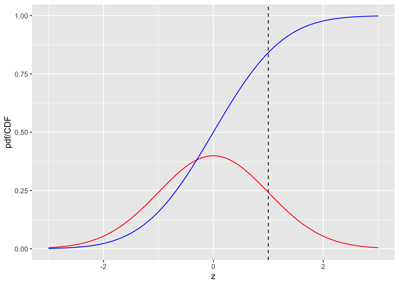
FIGURE 3.1: pdf-CDF plots for the unit normal distribution. The red curve is the pdf and the blue line is the CDF. The dashed line is the reporting threshold \(\zeta = 1\).
Fig. 3.1 shows plots, as functions of z, of the CDF and the pdf for the unit normal distribution. Since z-samples outside ±3 are unlikely, the plotted range, from -3 to +3 includes most of the distribution. The pdf is the familiar bell-shaped curve, centered at zero; the corresponding R function is dnorm() the density of the unit normal distribution. The CDF \(\Phi(z)\) increases monotonically from 0 to unity as z increases from \(-\infty\) to \(+\infty\). It is the sigmoid (S-shaped) shaped curve in Fig. 3.1; the corresponding R function is pnorm(). The dashed line corresponds to the reporting threshold \(\zeta = 1\). The area under the pdf to the left of \(\zeta\) equals the value of CDF at the selected \(\zeta\) (pnorm(1) = 0.841).
A related function is the inverse of Eqn. (3.6). Suppose the left hand side of Eqn. (3.6) is denoted \(p\), which is a probability in the range 0 to 1.
\[\begin{equation} p \equiv \Phi\left ( z \right )=\int_{-\infty }^{z}\phi(t)dt \tag{3.7} \end{equation}\]
The inverse of \(\Phi(z)\) is that function which when applied to \(p\) yields the upper limit \(z\) in Eqn. (3.7), i.e.,
\[\begin{equation} \Phi^{-1}(p) = z \tag{3.8} \end{equation}\]
Since \(p \equiv \Phi(z)\) it follows that
\[\begin{equation} \Phi(\Phi^{-1}(z))=z \tag{3.9} \end{equation}\]
This nicely satisfies the property of an inverse function. The inverse is known in statistical terminology as the quantile function, implemented in R as the qnorm(). Think of pnorm() as a probability and qnorm() as value on the z-axis.
To summarize the convention used in R, norm implies the unit normal distribution, p denotes a probability distribution function or CDF, q denotes a quantile function and d denotes a density function.
qnorm(0.025)
#> [1] -1.959964
qnorm(1-0.025)
#> [1] 1.959964
pnorm(qnorm(0.025))
#> [1] 0.025
qnorm(pnorm(-1.96))
#> [1] -1.96
Line 1 demonstrates the identity:
\[\begin{equation} \Phi^{-1}(0.025)=-1.959964 \tag{3.10} \end{equation}\]
Line 3 demonstrates the identity:
\[\begin{equation} \Phi^{-1}(1-0.025)=+1.959964 \tag{3.11} \end{equation}\]
Lines 5 and 7 demonstrate that pnorm and qnorm, applied in either order, are inverses of each other.
Eqn. (3.10) means that the (rounded) value -1.96 is such that the area under the pdf to the left of this value is 0.025. Similarly, Eqn. (3.11) means that the (rounded) value +1.96 is such that the area under the pdf to the left of this value is 1-0.025 = 0.975. In other words, -1.96 captures, to its left, the 2.5th percentile of the unit-normal distribution, and 1.96 captures, to its left, the 97.5th percentile of the unit-normal distribution, Fig. 3.2. Since between them they capture 95 percent of the unit-normal pdf, these two values can be used to estimate 95 percent confidence intervals.
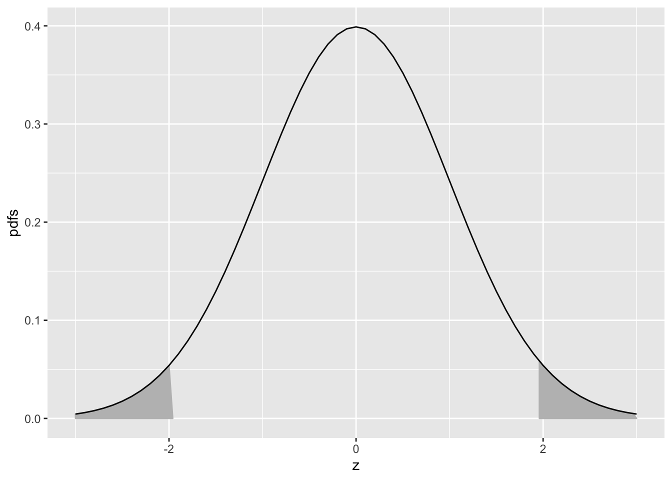
FIGURE 3.2: Illustrating that 95 percent of the total area under the unit normal pdf is contained in the range |z| < 1.96; this is used to construct a 95 percent confidence interval for an estimate of a suitably normalized statistic. The area in each shaded tail is 0.025.
If one knows that a variable is distributed as a unit-normal random variable, then the observed value minus 1.96 defines the lower limit of its 95 percent confidence interval, and the observed value plus 1.96 defines the upper limit of its 95 percent confidence interval.
3.8 Analytic expressions for specificity and sensitivity
Specificity corresponding to threshold \(\zeta\) is the probability that a Z-sample from a non-diseased case is smaller than \(\zeta\). By definition, this is the CDF corresponding to the threshold \(\zeta\). In other words:
\[\begin{equation} \left. \begin{aligned} Sp\left ( \zeta \right ) \equiv& P\left ( Z_{k_11} < \zeta\mid Z_{k_11} \sim N\left ( 0,1 \right )\right ) \\ =& \Phi\left ( \zeta \right ) \end{aligned} \right \} \tag{3.12} \end{equation}\]
The expression for sensitivity can be derived. Consider that the random variable obtaining by shifting the origin to \(\mu\). A little thought should convince the reader that \(Z_{k_22}-\mu\) is distributed as \(N(0,1)\). Therefore, the desired probability is:
\[\begin{equation} \left. \begin{aligned} Se\left ( \zeta \right ) \equiv& P\left ( Z_{k_22} \geq \zeta\right ) \\ =&P\left (\left ( Z_{k_22} -\mu \right ) \geq\left ( \zeta -\mu \right )\right ) \\ =&1-P\left (\left ( Z_{k_22} -\mu \right ) < \left ( \zeta -\mu \right )\right ) \\ =& 1-\Phi\left ( \zeta -\mu \right ) \end{aligned} \right \} \tag{3.13} \end{equation}\]
A little thought, based on the definition of the CDF function and the symmetry of the unit-normal pdf function, should convince the reader that:
\[\begin{equation} \left. \begin{aligned} 1-\Phi(\zeta)=& -\Phi(\zeta)\\ 1-\Phi(\zeta-\mu) =& \Phi(\mu-\zeta) \end{aligned} \right \} \tag{3.14} \end{equation}\]
Instead of carrying the “1 minus” around one can use the more compact notation. Summarizing, the analytical formulae for the specificity and sensitivity for the equal-variance binormal model are:
\[\begin{equation} Sp\left ( \zeta \right ) = \Phi(\zeta)\\ Se\left ( \zeta \right ) = \Phi(\mu-\zeta) \tag{3.15} \end{equation}\]
In Eqn. (3.15) the threshold \(\zeta\) appears with different signs because specificity is the area under a pdf to the left of the threshold while sensitivity is the area to the right.
Sensitivity and specificity are restricted to the range 0 to 1. The observer’s performance could be characterized by specifying sensitivity and specificity, i.e., a pair of numbers. If both sensitivity and specificity of an imaging system are greater than the corresponding values for another system, then the first system is unambiguously better than the second. But if sensitivity is greater for the first but specificity is greater for the second the comparison is ambiguous. A scalar measure is desirable that combines sensitivity and specificity into a single measure of diagnostic performance.
The parameter \(\mu\) satisfies the requirements of a scalar performancer measure, termed a figure of merit (FOM). Eqn. (3.15) can be solved for \(\mu\) as follows. Inverting the equations yields:
\[\begin{equation} \left. \begin{aligned} \zeta =&\Phi^{-1} \left (\text{Sp}\left ( \zeta \right ) \right )\\ \mu - \zeta =& \Phi^{-1} \left (\text{Se}\left ( \zeta \right ) \right ) \end{aligned} \right \} \tag{3.16} \end{equation}\]
Eliminating \(\zeta\) yields:
\[\begin{equation} \left. \begin{aligned} \mu =& \Phi^{-1} \left (\text{Sp}\left ( \zeta \right ) \right ) + \Phi^{-1} \left (\text{Se}\left ( \zeta \right ) \right ) \end{aligned} \right \} \tag{3.17} \end{equation}\]
This is a useful relation, as it converts a pair of numbers into a scalar performance measure. Now it is almost trivial to compare two modalities: the one with the higher \(\mu\) is better. In reality, the comparison is not trivial since like sensitivity and specificity \(\mu\) has to be estimated from a finite dataset and one must account for sampling variability.
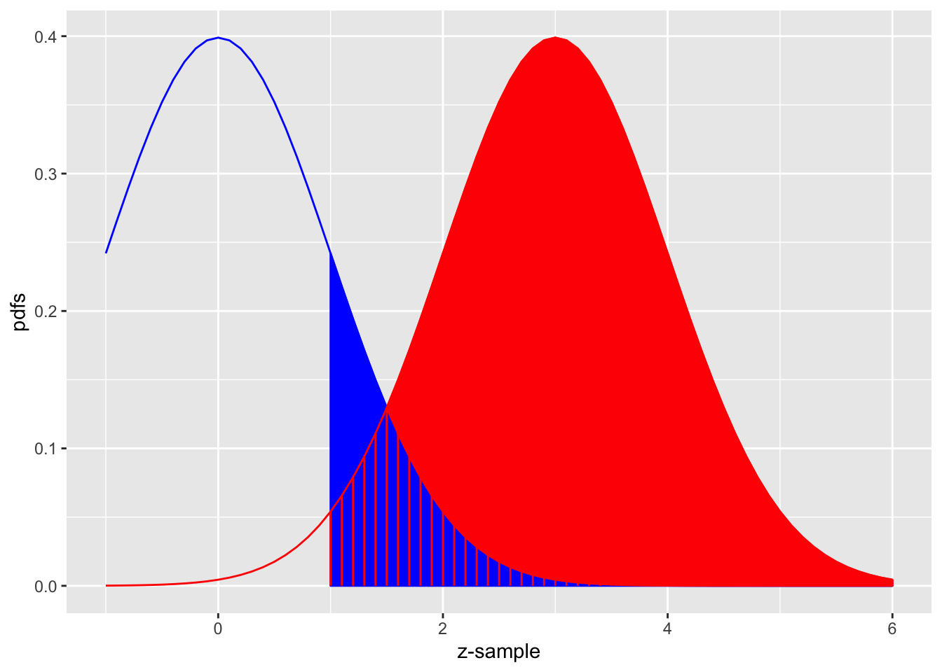
FIGURE 3.3: The equal-variance binormal model for \(\mu = 3\) and \(\zeta = 1\); the blue curve, centered at zero, is the pdf of non-diseased cases and the red one, centered at \(\mu = 3\), is the pdf of diseased cases. The left edge of the blue shaded region represents the threshold \(\zeta = 1\). The red shaded area including the common portion with the vertical red lines is sensitivity. The blue shaded area including the common portion with the vertical red lines is 1-specificity.
Fig. 3.3 shows the equal-variance binormal model for \(\mu = 3\) and \(\zeta = 1\). The blue-shaded area, including the “common” portion with the vertical red lines, is the probability that a z-sample from a non-diseased case exceeds \(\zeta = 1\), which is the complement of specificity, i.e., false positive fraction, which is 1 - pnorm(1) = 0.159. The red shaded area, including the “common” portion with the vertical red lines, is the probability that a z-sample from a diseased case exceeds \(\zeta = 1\), which is sensitivity or true positive fraction, which is pnorm(3-1)= 0.977.
See Appendix 3.14 for a demonstration of the concepts of sensitivity and specificity using R.
3.9 Inverse variation of sensitivity and specificity
The variation of sensitivity and specificity is modeled in the binormal model by the threshold parameter \(\zeta\). From Eqn. (3.12) specificity at threshold \(\zeta\) is \(\text{Sp} = \Phi(\zeta)\) and sensitivity is \(\text{Se} = \Phi(\mu-\zeta)\). Since the threshold \(\zeta\) appears with different signs the dependence of sensitivity on \(\zeta\) will be the opposite of that of specificity. In Fig. 3.3, the left edge of the blue shaded region represents the threshold \(\zeta = 1\). As \(\zeta = 1\) is moved towards the left, specificity decreases but sensitivity increases. Specificity decreases because less of the non-diseased distribution lies to the left of the lowered threshold, in other words fewer non-diseased cases are correctly diagnosed as non-diseased. Sensitivity increases because more of the diseased distribution lies to the right of the lowered threshold, in other words more diseased cases are correctly diagnosed as diseased.
If Observer 1 has higher sensitivity than Observer 2 but lower specificity it is difficult to unambiguously compare them; it is not impossible (Skaane et al. 2013). The unambiguous comparison is difficult for the following reason: assuming the Observer 2 can be coaxed into adopting a lower threshold, thereby decreasing specificity to match that of Observer 1 then it is possible that the Observer 2’s sensitivity, formerly smaller, could (and here is the ambiguity because if might not happen) now be greater than that of Observer 1.
A single figure of merit is desirable to the sensitivity - specificity analysis. It is possible to leverage the inverse variation of sensitivity and specificity by combing them into a single scalar measure, as was done with the \(\mu\) parameter in the previous section, Eqn. (3.17).
An equivalent way is by using the area under the ROC plot, discussed next.
3.10 The ROC curve
The receiver operating characteristic (ROC) is defined as the plot of sensitivity (y-axis) vs. 1-specificity (x-axis). Equivalently, it is the plot of TPF (y-axis) vs. FPF (x-axis). From Eqn. (3.15) it follows that:
\[\begin{equation} \left. \begin{aligned} \text{FPF}\left ( \zeta \right ) &\equiv 1 - \text{Sp}\left ( \zeta \right ) \\ &=\Phi\left ( -\zeta \right )\\ \text{TPF}\left ( \zeta \right ) &\equiv \text{Se}\left ( \zeta \right ) \\ &=\Phi\left (\mu -\zeta \right )\\ \end{aligned} \right \} \tag{3.18} \end{equation}\]
Specifying \(\zeta\) selects a particular operating point on this curve and varying \(\zeta\) from \(+\infty\) to \(-\infty\) causes the operating point to trace out the ROC curve from the origin (0,0) to (1,1). Note that as \(\zeta\) increases the operating point moves down the curve. The operating point \(O(\zeta|\mu)\) for the equal variance binormal model is:
\[\begin{equation} O\left ( \zeta \mid \mu \right ) = \left ( \Phi(-\zeta), \Phi(\mu-\zeta) \right ) \\ \tag{3.19} \end{equation}\]
The operating point predicted by the above equation lies exactly on the theoretical ROC curve. This condition can only be achieved with very large numbers of cases. With finite datasets the operating point will almost never be exactly on the theoretical curve.
The ROC curve is the locus of the operating point for fixed \(\mu\) and variable \(\zeta\). Fig. 3.4 shows examples of equal-variance binormal model ROC curves for different values of \(\mu\). Each has the property that TPF is a monotonically increasing function of FPF and the slope decreases monotonically as the operating point moves up the curve. As \(\mu\) increases the curves get progressively upward-left shifted, approaching the top-left corner of the ROC plot. In the limit \(\mu = \infty\) the curve degenerates into two line segments, a vertical one connecting the origin to (0,1) and a horizontal one connecting (0,1) to (1,1) – the ROC plot for a perfect observer.
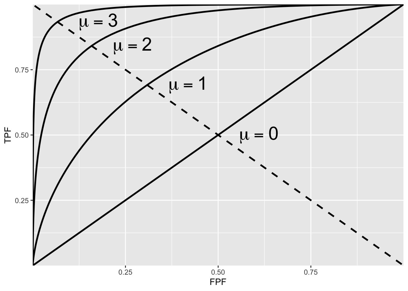
FIGURE 3.4: ROC plots predicted by the equal variance binormal model for different values of \(\mu\). As \(\mu\) increases the intersection of the curve with the negative diagonal moves closer to the ideal operating point, (0,1) at which sensitivity and specificity are both equal to unity.
3.10.1 The chance diagonal
In Fig. 3.4 the ROC curve for \(\mu=0\) is the positive diagonal of the ROC plot, termed the chance diagonal. Along this curve \(\text{TPF = FPF}\) and the observer’s performance is at chance level. For \(\mu=0\) the pdf of the diseased distribution is identical to that of the non-diseased distribution: both are centered at the origin. Therefore, no matter the choice of threshold \(\zeta\), \(\text{TPF = FPF}\). Setting \(\mu=0\) in Eqn. (3.18) yields:
\[\text{TPF}\left ( \zeta \right )=\text{FPF}\left ( \zeta \right )=\Phi\left ( -\zeta \right )\] In this case the red and blue curves in Fig. 3.3 coincide. The observer is unable to find any difference between the two distributions. This can happen if the cancers are of such low visibility that diseased cases are indistinguishable from non-diseased ones, or the observer’s skill level is so poor that the observer is unable to make use of distinguishing characteristics between diseased and non-diseased cases that do exist and which experts exploit.
3.10.2 The guessing observer
If the cases are indeed impossibly difficult and/or the observer has zero skill at discriminating between them, the observer has no option but to guess. This rarely happens in the clinic, as too much is at stake and this paragraph is intended to make a pedagogical point: the observer can move the operating point along the change diagonal. If there is no special incentive, the observer tosses a coin and if the coin lands head up, the observer states: “case is diseased” and otherwise states: “case is non-diseased”. When this procedure is averaged over many non-diseased and diseased cases, it will result in the operating point (0.5, 0.5). 5 To move the operating point downward, e.g., to (0.1, 0.1) the observer randomly selects an integer number between 1 and 10, equivalent to a 10-sided “coin”. Whenever a one “shows up”, the observer states “case is diseased” and otherwise the observer states “case is non-diseased”. To move the operating point to (0.2, 0.2) whenever a one or two “shows up”, the observer states “case is diseased” and otherwise the observer states “case is non-diseased”. One can appreciate that simply by changing the probability of stating “case is diseased” the observer can place the operating point anywhere on the chance diagonal but wherever the operating point is placed, it will satisfy TPF = FPF.
3.10.3 Symmetry with respect to negative diagonal
A characteristic of the ROC curves shown in Fig. 3.4 is that they are symmetric with respect to the negative diagonal, i.e., the line joining (0,1) and (1,0) which is shown as the dotted straight line in Fig. 3.4. The symmetry property is due to the equal variance nature of the binormal model and is not true for models considered in later chapters. The intersection between the ROC curve and the negative diagonal corresponds to \(\zeta = \mu/2\), in which case the operating point is:
\[\begin{equation} \left. \begin{aligned} \text{FPF}\left ( \zeta \right ) &=\Phi\left ( -\mu/2 \right )\\ \text{TPF}\left ( \zeta \right ) &=\Phi\left (\mu/2 \right )\\ \end{aligned} \right \} \tag{3.20} \end{equation}\]
The first equation implies:
\[1-\text{FPF}\left ( \zeta \right ) =1-\Phi\left ( -\mu/2 \right )= \Phi\left ( \mu/2 \right )\]
Therefore,
\[\begin{equation} \text{TPF}\left ( \zeta \right ) = 1-\text{FPF}\left ( \zeta \right ) \tag{3.21} \end{equation}\]
This equation describes a straight line with unit intercept and slope equal to minus 1, which is the negative diagonal. Since \(\text{TPF = Se}\) and \(\text{FPF = 1-Sp}\) another way of stating this is that at the intersection with the negative diagonal sensitivity equals specificity.
3.10.4 Area under the ROC curve
The area AUC (abbreviation for area under curve) under the ROC curve suggests itself as a measure of performance that is independent of threshold and therefore circumvents the ambiguity issue of comparing sensitivity/specificity pairs, and has other advantages.
It is defined by the following integrals:
\[\begin{equation} \begin{aligned} A_{z;\sigma = 1} &= \int_{0}^{1}TPF(\zeta)d(FPF(\zeta))\\ &=\int_{0}^{1}FPF(\zeta)d(TPF(\zeta))\\ \end{aligned} \tag{3.22} \end{equation}\]
Eqn. (3.22) has the following equivalent interpretations:
The first form performs the integration using thin vertical strips, e.g., extending from x to x + dx, where x is a temporary symbol for FPF. The area can be interpreted as the average TPF over all possible values of FPF.
The second form performs the integration using thin horizontal strips, e.g., extending from y to y + dy, where y is a temporary symbol for TPF. The area can be interpreted as the average FPF over all possible values of TPF.
By convention, the symbol \(A_z\) is used for the area under the unequal-variance binormal model predicted ROC curve. The more expressive term area under curve or AUC is used to include this and other methods of estimating the area under the ROC curve.
In Eqn. (3.22), the extra subscript \(\sigma = 1\) is necessary to distinguish it from another that corresponding to the unequal variance binormal model to be derived later. It can be shown that:
\[\begin{equation} A_{z;\sigma = 1} = \Phi\left ( \frac{\mu} {\sqrt{2}} \right ) \tag{3.23} \end{equation}\]
Since the ROC curve is bounded by the unit square, \(A_z\) must be between zero and one. If \(\mu\) is non-negative, \(A_{z;\sigma = 1}\) must be between 0.5 and 1. The chance diagonal, corresponding to \(\mu = 0\), yields \(A_{z;\sigma = 1} = 0.5\), while the perfect ROC curve, corresponding to \(\mu = \infty\) yields \(A_{z;\sigma = 1} = 1\).
Since it is a scalar quantity, \(A_z\) can be used to unambiguously quantify performance than is possible using sensitivity - specificity pairs.
3.10.5 Properties of the equal-variance binormal model ROC curve
The ROC curve is completely contained within the unit square. This follows from the fact that both axes of the plot are probabilities.
The operating point rises monotonically from (0,0) to (1,1).
Since \(\mu\) is positive, the slope of the equal-variance binormal model curve at the origin (0,0) is infinite and the slope at (1,1) is zero, and the slope along the curve is always non-negative and decreases monotonically as the operating point moves up the curve.
\(A_z\) is a monotone increasing function of \(\mu\). It varies from 0.5 to 1 as \(\mu\) varies from zero to infinity.
3.10.6 Comments
Property 2: since the operating point can both be expressed in terms of \(\Phi\) functions, which are monotone in their arguments, and in each case the argument \(\zeta\) appears with a negative sign it follows that as \(\zeta\) is lowered both TPF and FPF increase. The operating point corresponding to \(\zeta - d\zeta\) is to the upper right of that corresponding \(\zeta\) to (assuming \(d\zeta > 0\)).
Property 3: The slope of the ROC curve can be derived by differentiation (\(\mu\) is constant):
\[\begin{equation} \left. \begin{aligned} \frac{d(TPF)}{d(FPF)}&=\frac{d(\Phi(\mu-\zeta))}{d(\Phi(-\zeta))}\\ &=\frac{\phi(\mu-\zeta)}{\phi(-\zeta)}\\ &=\exp(\mu(\zeta-\mu/2)) \propto \exp(\mu \zeta)\\ \end{aligned} \right \} \tag{3.24} \end{equation}\]
The above derivation uses the fact that the differential of the CDF function yields the pdf function, i.e.,
\[d\Phi(\zeta)=P\left ( \zeta < Z < \zeta + d \zeta \right ) = \phi(\zeta)d\zeta\]
Since the slope of the ROC curve can be expressed as a power of \(e\) it is always non-negative. Provided \(\mu > 0\), in the limit \(\zeta\rightarrow \infty\) the slope at the origin approaches \(\infty\). Eqn. (3.24) also implies that in the limit \(\zeta\rightarrow -\infty\) the slope of the ROC curve at the end-point (1,1) approaches zero, i.e., the slope is a monotone increasing function of \(\zeta\). As \(\zeta\) decrease from \(+\infty\) to \(-\infty\), the slope decreases monotonically from \(+\infty\) to 0.
Fig. 3.5 is the ROC curve for the equal-variance binormal model for \(\mu = 3\). The entire curve is defined by varying \(\zeta\). Specifying a particular value of \(\zeta\) corresponds to specifying a particular point on the ROC curve. In Fig. TBA 3.5 the open circle corresponds to the operating point (0.159, 0.977) defined by \(\zeta = 1\): pnorm(-1) = 0.159; pnorm(3-1) = 0.977. The operating point lies exactly on the curve as this is a predicted operating point.
FIGURE 3.5: ROC curve predicted by equal variance binormal model for \(\mu = 3\). The circled operating point corresponds to \(\zeta = 1\). The operating point falls exactly on the curve, as these are analytical curves. With finite numbers of cases this is not observed in practice.
3.10.7 Physical interpretation of the mu-parameter
The \(\mu\) parameter is equivalent (Macmillan and Creelman 2004) to a signal detection theory variable denoted \(d'\) in the literature (pronounced “dee-prime”). It can be thought of as the perceptual signal to noise ratio (pSNR) of diseased cases relative to non-diseased ones. It is a measure of reader expertise and / or ease of detectability of the disease. SNR is a term widely used in engineering, specifically in signal detection theory (Green, Swets, et al. 1966; Egan 1975a). It dates to the early 1940s when one had the problem Jess Marcum (1960) of detecting faint radar reflections from a plane against a background of noise. The radar radio “receiver” is the origin of the term in Receiver Operating Characteristic.
The reader may be aware of the “rule-of-thumb” that if SNR exceeds three the target is likely to be detected. It will be shown later that the area under the ROC curve is the probability that a diseased case Z-sample is greater than that of a non-diseased one. The following code snippet shows that for \(\mu = 3\), the probability of detection is 98.3 percent.
#> pnorm(3/sqrt(2)) = 0.983For electrical signals, SNR can be measured with instruments but, in the context of decisions made by humans, what is measured is the perceptual SNR. Physical characteristics that differentiate non-diseased from diseased cases, and how well they are displayed will affect it; in addition the eye-sight of the observer is an obvious factor; not so obvious is how information is processed by the cognitive system, and the role of the observer’s expertise.
To this day I find it remarkable that an objective SNR-like quantity can be teased out of subjective observer decisions.
3.11 Confidence intervals for an operating point
A \((1-\alpha)\) confidence interval (CI) of a statistic is the range that is expected to contain the true value with probability \((1-\alpha)\).
It should be clear that a 99 percent CI is wider than a 95 percent CI, and that a 90 percent CI is narrower; in general, the higher the confidence that the interval contains the true value, the wider the range of the CI.
Calculation of a parametric confidence interval requires a distributional assumption (non-parametric estimation methods, which use resampling methods, are described later). With a distributional assumption the parameters of the distribution can be estimated and since the distribution accounts for variability, the needed confidence interval estimate follows.
With TPF and FPF, each of which involves a ratio of two integers, it is convenient to assume a binomial distribution for the following reason:
The diagnosis “non-diseased” vs. “diseased” represents a Bernoulli trial, i.e., one whose outcome is binary.
A Bernoulli trial is like a coin-toss, a special coin whose probability of landing “diseased” face up is \(p\) which is not necessarily 0.5 as with a real coin.
It is a theorem in statistics that the total number of Bernoulli outcomes of one type, e.g., \(n(FP)\), is a binomial-distributed random variable, with success probability \(\widehat{FPF}\) and trial size \(K_1\).
\[\begin{equation} n(FP) \sim B\left ( K_1, \widehat{FPF} \right ) \tag{3.25} \end{equation}\]
\(B(n,p)\) denotes the binomial distribution with success probability \(p\) and trial size \(n\):
\[\begin{equation} \left. \begin{aligned} k \sim& B\left ( n, p \right )\\ k=& 0,1,2,...,n\\ \end{aligned} \right \} \tag{3.26} \end{equation}\]
Eqn. (3.26) states that \(k\) is a random sample from the binomial distribution \(B(n,p)\). For reference, the probability mass function \(\text{pmf}\) of \(B(n,p)\) is defined by (the subscript \(Bin\) denotes a binomial distribution):
\[\begin{equation} \text{pmf}_{Bin}\left ( k;n,p \right )=\binom{n}{k}p^k(1-p)^{n-k} \tag{3.27} \end{equation}\]
For a discrete distribution, one has probability mass function in contrast to a continuous distribution where one has a probability density function.
The binomial coefficient \(\binom{n}{k}\) appearing in Eqn. (3.27), to be read as “\(n\) pick \(k\)”, is defined by:
\[\begin{equation} \binom{n}{k}=\frac{n!}{k!(n-k)!} \tag{3.28} \end{equation}\]
From the properties of the binomial distribution the variance of n(FP) is given by:
\[\begin{equation} \sigma_{n(FP)}^2=K_1\widehat{\text{FPF}}\left ( 1 - \widehat{\text{FPF}} \right ) \tag{3.29} \end{equation}\]
It follows that \(\text{FPF}\) has mean \(\widehat{\text{FPF}}\) and variance \(\sigma_{\text{FPF}}^2\) given by (since \(Var(aX) = a^2 Var(X)\) where \(a\) is a constant):
\[\begin{equation} \sigma_{\text{FPF}}^2 = \frac{\widehat{\text{FPF}}\left ( 1 - \widehat{\text{FPF}} \right )}{K_1} \tag{3.30} \end{equation}\]
For large \(K_1\) the distribution of \(\text{FPF}\) approaches a normal distribution:
\[\begin{equation} \left. \begin{aligned} FPF \sim N\left ( \widehat{\text{FPF}}, \sigma_{\text{FPF}}^2 \right )\end{aligned} \right \} \tag{3.31} \end{equation}\]
Eqn. (3.31) allows us to write down the approximate symmetric confidence interval for \(\widehat{\text{FPF}}\), i.e., \(\pm z_{\alpha/2} \times \sigma_{\text{FPF}}\) around \(\widehat{\text{FPF}}\).
\[\begin{equation} CI_{1-\alpha}^{\text{FPF}}=\left ( \widehat{\text{FPF}} - z_{\alpha/2} \sigma_{\text{FPF}}, \widehat{\text{FPF}} + z_{\alpha/2} \sigma_{\text{FPF}} \right ) \tag{3.32} \end{equation}\]
In Eqn. (3.32) \(z_{\alpha/2}\) is the upper \(\alpha/2\) quantile of the unit normal distribution: it is defined such that the area to the right under the unit normal distribution pdf from \(z_{\alpha/2}\) to \(+\infty\) equals \(\alpha/2\). For example \(z_{0.025} = 1.96\), see Fig. 3.2. In general \(z_{\alpha/2} = -\Phi^{-1}(\alpha/2)\). For example -qnorm(0.025) = 1.96.
These relations involving \(z_{\alpha/2}\) follow:
\[\begin{equation} \left. \begin{aligned} z_{\alpha/2} &=\Phi^{-1}\left ( 1-\alpha/2 \right )\\ &= - \Phi^{-1}\left (\alpha/2 \right )\\ \alpha/2&=\int_{z_{\alpha/2}}^{\infty}\phi(z)dz\\ &= 1-\Phi(z_{\alpha/2})\\ &= \Phi(-z_{\alpha/2})\\ \end{aligned} \right \} \tag{3.33} \end{equation}\]
The normal approximation is adequate if both of the following two conditions are both met: \(K_1\widehat{FPF} > 10\) and \(K_1(1-\widehat{\text{FPF}}) > 10\). This means, approximately, that \(\widehat{\text{FPF}}\) cannot be too close to zero or 1.
Similarly, an approximate symmetric \((1-\alpha)\) confidence interval for \(\text{TPF}\) is:
\[\begin{equation} CI_{1-\alpha}^{\text{TPF}}=\left ( \widehat{\text{TPF}} - z_{\alpha/2} \sigma_{\text{TPF}}, \widehat{\text{TPF}} + z_{\alpha/2} \sigma_{\text{TPF}} \right ) \tag{3.34} \end{equation}\]
In Eqn. (3.34),
\[\begin{equation} \sigma_{\text{TPF}}^2 = \frac{\widehat{\text{TPF}}\left ( 1 - \widehat{\text{TPF}} \right )}{K_2} \tag{3.35} \end{equation}\]
The confidence intervals are largest when the probabilities (FPF or TPF) are close to 0.5 and decrease inversely as the square root of the relevant number of cases. The symmetric binomial distribution based estimates can stray outside the allowed range (0 to 1). Exact confidence intervals that are asymmetric around the central value and which are guaranteed to be in the allowed range can be calculated: it is implemented in R in function binom.test()and used below:
#> alpha =  0.05
#> K1 =  99
#> K2 =  111
#> mu =  5
#> zeta =  2.5
#> Specificity =  0.99
#> Sensitivity =  0.991
#> Approx 95 percent CI for Specificity =  0.97 1.01
#> Exact 95 percent CI for Specificity =  0.945 1
#> Approx 95 percent CI for Sensitivity =  0.973 1.01
#> Exact 95 percent CI for Sensitivity =  0.951 1
Note that the approximate confidence intervals can stray outside the allowed range but the exact confidence intervals do not.
3.12 Variability: the Beam study
In this study (Beam, Layde, and Sullivan 1996) fifty accredited mammography centers were randomly sampled in the United States. “Accredited” is a legal/regulatory term implying, among other things, that the radiologists interpreting the breast cases were “board certified” by the American Board of Radiology. One hundred eight (108) certified radiologists from these centers gave blinded interpretation to a common set of 79 randomly sampled (stratified sampling) enriched screening cases containing 45 cases with cancer and the rest with benign lesions. Ground truth for these women had been established either by biopsy or by 2-year follow-up.
The observed range of sensitivity (TPF) was 53 percent and the range of FPF was 63 percent; the corresponding range for the AUC was 21 percent, Table 3.1. Empirical AUC was estimated using a 5-point BIRADS ratings of the images (the zero category was not allowed). Explanation of empirical AUC is deferred to Chapter 5.
| Min | Max | Range | |
|---|---|---|---|
| Sensitivity | 46.70 | 100.00 | 53.30 |
| Specificity | 36.30 | 99.30 | 63.00 |
| AUC | 0.74 | 0.95 | 0.21 |
FIGURE 3.6: Schematic patterned from the Beam et al study showing the ROC operating points of 108 mammographers. Wide variability in sensitivity and specificity are evident while AUC is less variable. See text below.
In Fig. 3.6 if one looks at the points labeled (B) and (C) one can mentally construct a smooth ROC curve that starts at (0,0), passes roughly through these points and ends at (1,1). In this sense, the intrinsic performances (i.e., AUCs or equivalently the \(\mu\) parameters) of radiologists B and C are similar. The only difference between them is that radiologist B is using lower threshold than radiologist C. Radiologist C is more concerned with minimizing FPs while radiologist B is more concerned with maximizing sensitivity. By appropriate feedback radiologist C can perhaps be induced to change the threshold to that of radiologist B. An example of feedback might be: “you are missing too many cancers and this could get us all into trouble; worry less about reduced specificity and more about increasing your sensitivity”.
In contrast, radiologist A has intrinsically superior performance to B or C. No change in threshold is going to get the other two to a similar level of performance as radiologist A. Extensive training will be needed to bring the under-performing radiologists to the expert level of radiologist A.
Fig. 3.6 and Table 3.1 illustrate several important principles.
Since an operating point is characterized by two values, unless both numbers are higher (e.g., radiologist A vs. B or C) it is difficult to unambiguously compare them.
While sensitivity and specificity depend on the reporting threshold, the area under the ROC plot is independent of it. Using the area under the ROC curve one can unambiguously compare two readers.
Combining sensitivity and the complement of specificity into a single AUC measure yields the additional benefit of lower variability. In Fig. 3.6, the range for sensitivity is 53 percent while that for specificity is 63 percent. In contrast, the range for AUC is only 21 percent. This means that much of the observed variations in sensitivity and specificity are due to variations in thresholds, and using AUC eliminates this source of variability. Decreased variability of a measure is a highly desirable characteristic as it implies the measurement is more precise making it easier to detect differences between readers.
3.13 Discussion
Sensitivity and specificity are widely used in the medical imaging literature. It is important to realize that they do not provide a complete picture of diagnostic performance, since they represent performance at a particular observer-dependent threshold. As demonstrated in Fig. 3.6 expert observers can and do operate at different thresholds. If using sensitivity and specificity the dependence on reporting threshold often makes it difficult to unambiguously compare observers. An additional source of variability is introduced by the varying thresholds.
The ROC curve and AUC are completely defined by the \(\mu\) parameter of the equal variance binormal model. Since both are independent of reporting threshold they overcome the ambiguity inherent in comparing sensitivity/specificity pairs. AUC is widely used in assessing imaging systems.
It should impress the reader that a subjective internal sensory perception of disease presence and an equally subjective internal threshold can be translated into an objective performance measure, such as the area under an ROC curve or equivalently, the \(\mu\) parameter. The latter has the physical meaning of a perceptual signal to noise ratio.
The properties of the unit normal distribution and the binomial distribution were used to derive parametric confidence intervals for sensitivity and specificity. These were compared to exact confidence intervals. An important study was reviewed showing wide variability in sensitivity and specificity for radiologists interpreting a common set of cases in screening mammography, but smaller variability in AUCs. This is because much of the variability in sensitivity and specificity is due to variation of the reporting threshold, which does not affect the area under the ROC curve. This is an important reason for preferring comparisons based on area under the ROC curve to those based on comparing sensitivity/specificity pairs.
3.14 Appendix I
3.14.1 Estimates from a finite sample
The following embedded code simulates 9 non-diseased and 11 diseased cases. The \(\mu\) parameter is 1.5 and \(\zeta\) is \(\mu/2\). Shown are the estimates of sensitivity and specificity and \(\mu\).
#> seed =  100
#> mu true =  1.5
#> zeta true =  0.75
#> K1 =  9
#> K2 =  11
#> Specificity =  0.889
#> Sensitivity =  0.909
#> Est. of mu =  2.56
Since this is a finite sample the estimate of \(\mu\) is not equal to the true value. In fact, all of the estimates, sensitivity, specificity and \(\mu\) are subject to sampling variability.
3.14.2 Changing the seed variable
No matter how many times one runs the above code, one always sees the same output shown above. This is because one sets the seed of the random number generator to a fixed value, namely 100. This is like having a perfectly reproducible reader repeatedly interpreting the same cases – one always gets the same results. Changing the seed to 101 yields:
#> seed =  101
#> mu true =  1.5
#> zeta true =  0.75
#> K1 =  9
#> K2 =  11
#> Specificity =  0.778
#> Sensitivity =  0.545
#> Est. of mu =  0.879
Changing seed is equivalent to sampling a completely new set of cases. The effect is quite large (estimated sensitivity falls from 0.909 to 0.545 and estimated \(\mu\) falls from 2.56 to 0.879) because the size of the relevant case set, \(K_2=11\) for sensitivity, is small.
3.14.3 Increasing the numbers of cases
Here we increase \(K_1\) and \(K_2\), by a factor of 10 each, and reset the seed to 100.
#> seed =  100
#> mu true =  1.5
#> zeta true =  0.75
#> K1 =  90
#> K2 =  110
#> Specificity =  0.778
#> Sensitivity =  0.836
#> Est. of mu =  1.74
Next we change seed to 101.
#> seed =  101
#> mu true =  1.5
#> zeta true =  0.75
#> K1 =  90
#> K2 =  110
#> Specificity =  0.811
#> Sensitivity =  0.755
#> Est. of mu =  1.57
Notice that now the values are less sensitive to seed. Table 3.2 illustrates this trend with increasing sample size.
| K1 | K2 | seed | Se | Sp | mu |
|---|---|---|---|---|---|
| 9 | 11 | 100 | 0.889 | 0.909 | 2.556 |
| 9 | 11 | 101 | 0.778 | 0.545 | 0.879 |
| 90 | 110 | 100 | 0.778 | 0.836 | 1.744 |
| 90 | 110 | 101 | 0.811 | 0.755 | 1.571 |
| 900 | 1100 | 100 | 0.764 | 0.761 | 1.430 |
| 900 | 1100 | 101 | 0.807 | 0.759 | 1.569 |
| 9000 | 11000 | 100 | 0.774 | 0.772 | 1.496 |
| 9000 | 11000 | 101 | 0.771 | 0.775 | 1.498 |
| Inf | Inf | NA | 0.773 | 0.773 | 1.500 |
As the numbers of cases increase, the sensitivity and specificity converge to a common value, around 0.773 and the estimate of the separation parameter converges to the known value.
Because the threshold is halfway between the two distributions, as in this example, sensitivity and specificity are identical. In words, with two unit variance distributions separated by 1.5, the area under the diseased distribution (centered at 1.5) above 0.75, namely sensitivity, equals the area under the non-diseased distribution (centered at zero) below 0.75, namely specificity, and the common value is \(\Phi(0.75)= 0.773\), yielding the last row of Table 3.2, and example 1 in the above code snippet. Example 2 in the above code snippet illustrates Eqn. (3.17). The factor of two arises since in this example sensitivity and specificity are identical.
From Table 3.2, for the same numbers of cases but different seeds, comparing pairs of sensitivity and specificity values is more difficult as two pairs of numbers (i.e., four numbers) are involved. Comparing a single pair of \(\mu\) values is easier as only two numbers are involved. The tendency of the pairs to become independent of case sample is discernible with fewer cases with \(\mu\), around 90/110 cases, than with sensitivity and specificity pairs.
The numbers in the table might appear disheartening in terms of the implied numbers of cases needed to detect a difference in specificity. Even with 200 cases, the difference in specificity for two seed values is 0.081, which is large considering that the scale extends from 0 to 1.0. A similar comment applies to differences in sensitivity. The situation is not quite that bad:
One uses an area measure that combines sensitivity and specificity and hence yields less variability. One uses the ratings paradigm which is more efficient than the binary paradigm used in this chapter. Finally, one takes advantage of correlations that exist between the interpretations using matched-case matched-reader interpretations in two modalities; this tends to decrease variability in the AUC-difference even further (most applications of ROC methods involved detecting differences in AUCs not absolute values).
REFERENCES
The \(-\infty\) to \(+\infty\) scale is not an assumption. The decision variable scale could just as well range from a to b, where a < b; with appropriate re-scaling of the decision variable, there will be no changes in the rank-orderings, and the scale can be made extend from \(-\infty\) to \(+\infty\).↩︎
Even if the experimenter attempts to deceive the radiologist, by claiming for example that there are roughly equal numbers of non-diseased and diseased cases, after interpreting a few tens of cases the radiologist will know that a deception is involved. Deception in such studies is not a good idea, as the observer’s performance is not being measured in a “steady state condition” – the observer’s performance will change as the observer “learns” the true disease prevalence.↩︎
If the common variance is not unity, one can re-scale the decision axis to achieve unit-variance without changing the predictions of the model.↩︎
Many cases are assumed as otherwise, due to sampling variability, the operating point will not be on the theoretical ROC curve.↩︎