Chapter 7 Proper ROC models
7.2 Introduction
The binormal model has been widely used to fit ROC datasets in a wide range of applications not limited to medical imaging. However, binormal model fits almost invariably lead to ROC curves that inappropriately cross the chance diagonal leading to a prediction of a region of the ROC curve where performance is worse than chance even for expert observers. By convention, such curves are termed “improper”. A chance line crossing near the upper right corner of the ROC plot occurs when \(b < 1\) and near the origin if \(b > 1\).
Since \(b\) is a continuous-variable parameter there is zero probability that an estimate of \(b\) will be exactly equal to one, the only condition under which there is no “hook”. Therefore, every fitted binormal model ROC curve is “improper”.
The improper behavior is often not readily visible. One may need to “zoom-in” on the upper-right corner to see it. Any fit that predicts worse than chance level performance anywhere on the ROC plot, visible or not, is scientifically indefensible. Much effort has gone into developing models that always predict proper ROC curves, i.e., those that do not cross the chance diagonal. These are called “proper” ROC curves (some of literature uses the quotes and some does not). There are at least four methods for fitting proper ROC curves, and these are listed in reverse chronological order.
The most recent (2016) one (DP Chakraborty and Svahn 2011; DP Chakraborty, Yoon, and Mello-Thoms 2012) is based on the radiological search model (RSM) and is implemented in the
RJafrocpackage.A method (Dorfman, Berbaum, and Brandser 2000; Dorfman and Berbaum 2000b, 2000a) based on the contaminated binormal model (CBM), available as part of DBM-MRMC software from a University of Iowa website and also implemented in the
RJafrocpackage.The binormal model-based proper ROC fitting algorithm (Charles E. Metz and Pan 1999; Pan and Metz 1997) developed by Metz and Pan implemented in PROPROC software available as part of DBM-MRMC software.
The bigamma model (Dorfman et al. 1997) fitting algorithm for which no software is currently readily available but it is fairly easy to implement.
LROCFIT, based on the location ROC (LROC) paradigm (Swensson 1996), which also predicts proper ROC curves, but the data has to be acquired according to the LROC paradigm while all of the other methods described in this chapter work with ROC data (no localization information).
A related issue is data degeneracy that occurs when a reader fails to provide an interior ROC point. The binormal model does not yield reasonable fits to such data and the researcher has no option but to discard the data or use the empirical AUC.
To understand how proper ROCs can be generated we need to understand a quantity called the likelihood ratio and the fact that slope of the ROC curve always equals the likelihood ratio, independent of parametric assumptions.
7.3 ROC slope equals likelihood ratio
According to the binormal model:
\[\begin{equation} \left.\begin{aligned} \text{FPF}&=\Phi\left( -z \right)\\ \text{TPF}&=\Phi\left( a-bz \right) \end{aligned} \right\} \tag{7.1} \end{equation}\]
The slope \(m\left( z|a,b \right)\) of the ROC curve is:
\[\begin{equation} \left.\begin{aligned} m\left( z|a,b \right)&=\frac{\frac{\partial \left( TPF \right)}{\partial z}}{\frac{\partial \left( FPF \right)}{\partial z}}\\ &=\frac{b\phi\left( a-bz \right)}{\phi\left( -z \right)}\\ &=b\exp\left( -\frac{\left( bz-a \right)^2 - z^2}{2} \right) \end{aligned}\right\} \tag{7.2} \end{equation}\]
The probability density functions (pdfs) for the binormal model were defined earlier and are reproduced here (N = non-diseased, D = diseased):
\[\begin{equation} \left.\begin{aligned} \text{pdf}_N\left( z \right) &= \frac{1}{\sqrt{2\pi}}\exp\left( -\frac{z^2}{2} \right) \\ \text{pdf}_D\left( z \right) &= \frac{b}{\sqrt{2\pi}}\exp\left( -\frac{\left( bz-a \right)^2}{2} \right) \\ \end{aligned}\right\} \tag{7.3} \end{equation}\]
The likelihood ratio is defined by (the subscript “BIN” is for “binormal model”):
\[\begin{equation} \left.\begin{aligned} l_{\text{BIN}}\left( z | a,b\right) &\equiv \frac{\text{pdf}_D\left( z \right)}{\text{pdf}_N\left( z \right)} \\ &= b\exp\left( -\frac{\left( bz-a \right)^2 -z^2}{2} \right) \\ \end{aligned}\right\} \tag{7.4} \end{equation}\]
It is seen from Eqn. (7.2) and Eqn. (7.4) that the likelihood ratio equals the slope of the ROC curve:
\[\begin{equation} l_{\text{BIN}}\left( z | a,b\right) = m\left( z | a,b\right) \tag{7.5} \end{equation}\]
While illustrated for the binormal model, this theorem is actually independent of any distributional assumptions (Egan 1975b). The reason for the name “likelihood ratio” is that early researchers in the field used the term “likelihood function” for what statisticians now term “probability density function”. Hence the ratio of two likelihood functions was termed a “likelihood ratio” when in fact it is a ratio of two pdfs.
7.4 The likelihood ratio observer maximizes AUC
An observer who maximizes TPF at each FPF for all values \(0 \le \text{FPF} \le 1\) is called a Neyman-Pearson observer (Neyman and Pearson 1933). It can be shown that the Neyman-Pearson observer uses the likelihood ratio as the decision variable (Green, Swets, et al. 1966).
A consequence is that AUC for a likelihood ratio observer represents an upper limit on performance, and such an observer is called an “ideal observer”. Moreover use of the likelihood ratio as the decision variable always yields proper ROC curves.
These statements call for an explanation.
7.4.1 Explanation
So far the decision rule has been that if the z-sample for a case satisfies \(z \ge \zeta\) the case is diagnosed as diseased and otherwise it is diagnosed as non-diseased.
The likelihood ratio involves a deeper concept. It is assumed that the observer knows the pdfs of non-diseased and diseased cases as functions of z. The observer computes the ratio \(l(z)\) at the observed z-sample. If \(l(z) \ge \lambda\) the case is diagnosed as diseased and otherwise the case is diagnosed as non-diseased. Note the difference:
Binormal model observer: \(z \ge \zeta\)
Likelihood ratio observer: \(l(z) \ge \lambda\)
A word on notation: when the decision variable was \(z\) I used the corresponding Greek character \(\zeta\) to denote a threshold on the z-axis. Since likelihood ratio is denoted \(l\), the corresponding Greek character is \(\lambda\).
The observer has transformed the decision variable \(z\) to a new variable \(l(z)\) and uses the new variable to make decisions. Varying \(\lambda\) allows the observer to generate the likelihood ratio ROC curve which is “proper”.
If the decision variable \(z\) results in improper ROC curves, as does the z-sample in the binormal model, the transformation will not be monotonic 11. If the transformation were monotonic, that would imply that z was already equivalent to the likelihood ratio.
To summarize these concepts the likelihood ratio observer transforms \(z\) to \(l(z)\):
\[\begin{equation} l\left( z \right) \equiv \frac{\text{pdf}_D\left( z \right)}{\text{pdf}_N\left( z \right)} \tag{7.6} \end{equation}\]
Then the decision variable \(M\left( l\left( z \right) \right)\) will yield a proper ROC curve. Here \(M\left( \right)\) is an arbitrary monotonic increasing function of its argument, i.e. if \(x_2 > x_1\):
\[\begin{equation} M\left( x_2 \right) \ge M\left( x_1 \right) \tag{7.7} \end{equation}\]
The transformation allows flat portions.
7.5 The likelihood ratio observer
An observer using the likelihood ratio or any monotonic transformation of it as the decision variable is termed a likelihood ratio observer.
In Fig. 7.1 plots A-F, all of which apply to \(a = 0.7\) and \(b = 0.5\), the ordinate is labeled \(\text{lr}\) for likelihood ratio.
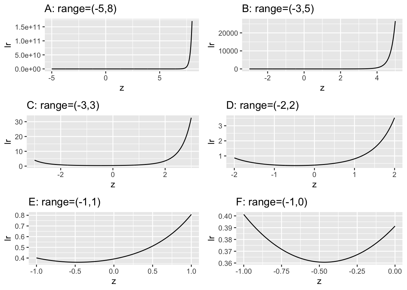
FIGURE 7.1: These plots of likelihood ratio \(\text{lr}\) of the ROC curves as functions of z for \(a = 0.7, b = 0.5\). They correspond to different ranges along the z-axis, starting with a ‘birds-eye’ view (panel A) and gradually focusing in on the region near the minimum (panel F).
Focusing on plot A in Fig. 7.1 in which range of z is -5 to 8, imagine a sliding threshold \(\lambda\) moving down along the ordinate, starting from very high values, \(\approx 1.5 \times 10^{11}\). The decision rule is to diagnose the case as “diseased” if \(\text{lr} \ge \lambda\), and otherwise the case is diagnosed as “non-diseased”. In plot A the likelihood ratio \(\text{lr}\) seems, for all practical purposes, to be monotonically related to z, so on the surface it makes no difference which decision rule is used, that based on \(\text{lr} \ge \lambda\) or that based on \(z \ge \zeta\). The same conclusion is reached for Plot B, which focuses on the range (-3,5). Plot C showing the range (-3,3) reveals the first hint of something different going on, for now the ordinate \(\text{lr}\) is not monotonically related to \(z\) since the \(\text{lr}\) function has a minimum. For \(\text{lr} > \approx 1\) there are two values of \(\zeta\) corresponding to a each value of \(\lambda\). This behavior is amplified in the remaining plots, as one “homes-in” on the minimum. Taking the clearest example, plot F, for \(\lambda = 0.37\) the two values are (-0.728, 0.206). These are denoted by \(\zeta_L=-0.728\) and \(\zeta_U=0.206\). The likelihood ratio observer using threshold \(\lambda=0.37\) declares all cases with \(\text{lr} \ge 0.37\) as diseased, and non-diseased otherwise. The corresponding z-sample binormal model observer must declare cases with \(z \ge \zeta_U\) and cases with \(z < \zeta_L\) as diseased, and non-diseased otherwise. The z-sample rule is more complicated and non-intuitive: why should cases with very low z-samples be declared diseased? The reason is that according to the z-sample based model assumed by the observer both very high and very low values of z are consistent with the case being diseased.
Since likelihood ratio decreases as one moves down the y-axis in Fig. 7.1) the slope of the likelihood ratio generated ROC curve decreases monotonically as the operating point moves up the curve. Since likelihood ratio is the ratio of two probabilities, it - and consequently the slope of the ROC - is always non-negative. This rules out chance line crossings and “hooks”. The likelihood ratio observer always generates a proper ROC curve.
Recall that the observer needs to know the two pdfs and compute a ratio based on the observed z-sample. Since the pdfs defined above were specific to the binormal model the likelihood ratio observer described above is, more carefully stated, a binormal-model-based likelihood ratio observer.
It can be shown that the likelihood ratio observer achieves the highest ROC curve (in the Neyman-Pearson sense) and consequently the highest AUC when compared to observers using other decision rules. In this sense the likelihood ratio observer is an ideal observer.
The observer can use a decision rule that is based on any monotonic increasing transformation of the likelihood ratio and the resulting ROC curve will be identical to that based on the likelihood ratio; the slope of the resulting curve always equals the likelihood ratio (i.e., before the monotonic transformation). For example, the monotonic transformation could yield a variable ranging from -infinity to plus infinity but the slope of the resulting ROC curve will still be that for the likelihood ratio observer prior to the transformation.
Since AUC of the likelihood ratio observer is optimal with respect to other observers using different decision rules or different underlying models of the decision variable, the AUC achieved by the likelihood ratio observer is unique regardless of the model used to fit the proper ROC curve. The shapes of the predicted proper ROC curves could be model dependent and differ from each other but the AUCs will all be the same. This is demonstrated in book Chapter TBA 18 for RSM, PROPROC and CBM models fitted to a large number of datasets.
7.6 PROPROC
An algorithm (Charles E. Metz and Pan 1999), based on the observer using the binormal model likelihood ratio, has been implemented. The software is called PROPROC, for proper ROC. 12
7.6.1 PROPROC formulae
The method uses two parameters \(c,d_a\) defined as follows:
\[\begin{equation} \left.\begin{aligned} c &= \frac{b-1}{b+1} \\ d_a &= \frac{\sqrt{2}a}{1+b^2} \\ \end{aligned}\right\} \tag{7.8} \end{equation}\]
Allowed values of the parameters are as follows:
\[\begin{equation} \left.\begin{aligned} & -1 < c < 1 \\ & 0 < d_a < \infty \\ \end{aligned}\right\} \tag{7.9} \end{equation}\]
Eqn. (7.8) can be solved for the \(a,b\) parameters as functions of the \(c.d_a\) parameters:
\[\begin{equation} \left.\begin{aligned} a &= \frac{d_a}{\sqrt{2}}\sqrt{1+{{\left( \frac{c+1}{c-1} \right)^2}}} \\ b &= -\frac{c+1}{c-1} \\ \end{aligned}\right\} \tag{7.10} \end{equation}\]
Since \(b < 1\) with most clinical datasets, one expects to find \(c < 0\). The proper ROC curve is defined by (Charles E. Metz and Pan 1999) (the threshold variable \(v\), which is the PROPROC analog of \(\zeta\), is defined below):
\[\begin{equation} \left.\begin{aligned} FPF\left( v \right) &= \Phi\left( -\left( 1-c \right)v -\frac{d_a}{2}\sqrt{1+c^2} \right) \\ &+\Phi\left( -\left( 1-c \right)v +\frac{d_a}{2c}\sqrt{1+c^2} \right) -H(c) \\ TPF\left( v \right) &= \Phi\left( -\left( 1+c \right)v +\frac{d_a}{2}\sqrt{1+c^2} \right) \\ &+\Phi\left( -\left( 1+c \right)v +\frac{d_a}{2c}\sqrt{1+c^2} \right) -H(c) \\ \end{aligned}\right\} \tag{7.11} \end{equation}\]
The (Heaviside) step function \(H(x)\) is defined by:
\[\begin{equation} \left.\begin{aligned} H\left( x < 0 \right) &= 0 \\ H\left( x > 0 \right) &= 1 \\ \end{aligned}\right\} \tag{7.12} \end{equation}\]
The function is discontinuous, but its value at \(x = 0\) is irrelevant because \(c = 0\) implies \(b = 1\), in which case the equal variance binormal model applies, which predicts proper ROCs.
Depending on the value of \(c\) the threshold variable \(v\) in Eqn. (7.11) has different ranges:
\[\begin{equation} \left.\begin{aligned} \begin{matrix} \frac{d_a}{4c}\sqrt{1+c^2} \le v \le \infty & \text{if} & c<0 \end{matrix}\\ \begin{matrix} -\infty \le v \le \infty & \text{if} & c=0 \end{matrix}\\ \begin{matrix} -\infty \le v \le\frac{d_a}{4c}\sqrt{1+c^2} \le v & \text{if} & c<0 \end{matrix}\\ \\ \end{aligned}\right\} \tag{7.13} \end{equation}\]
PROPROC software implements a maximum likelihood method to estimate the \(c, d_a\) parameters from ratings data. The 1999 publication (Charles E. Metz and Pan 1999) states, without proof, that the area under the proper ROC is give by:
\[\begin{equation} A_{\text{prop}}=\Phi\left( \frac{d_a}{\sqrt{2}} \right) + 2F\left\{-\frac{d_a}{\sqrt{2}},0;-\frac{1-c^2}{1+c^2} \right\} \tag{7.14} \end{equation}\]
Here \(F(X,Y;\rho)\) is the bivariate standard-normal (i.e., zero means and unit variances) cumulative distribution function (CDF) with correlation coefficient \(\rho\). In the notation of book Chapter 21:
\[\begin{equation} F\left( X,Y;\rho \right)=\int_{x=-\infty}^{X} \int_{y=-\infty}^{Y} dx dy ~ ~ f\left( \left( \begin{matrix} x \\ y \end{matrix} \right) \bigg\rvert \left( \begin{matrix} 0 \\ 0 \end{matrix} \right), \left( \begin{matrix} 1 & \rho \\ \rho & 1 \end{matrix} \right) \right) \tag{7.15} \end{equation}\]
Here \(f\) is the pdf of a standard-normal bivariate distribution with correlation \(\rho\), i.e., the mean is the zero column vector of length 2 and the 2 x 2 covariance matrix has ones along the diagonal and \(\rho\) along the off-diagonal.
The first term in Eqn. (7.14) is equal to the area under the binormal model ROC curve Eqn. (6.19). Therefore,
\[\begin{equation} A_{\text{prop}}=A_z+2F\left( -\frac{d_a}{\sqrt{2}},0;-\frac{1-c^2}{1+c^2} \right) \tag{7.16} \end{equation}\]
Since F (a CDF, which is a probability) is non-negative,
\[\begin{equation} A_{\text{prop}}\ge A_z \tag{7.17} \end{equation}\]
This reinforces the result stated earlier.
7.6.2 PROPROC code implementation
Here is the code to generate PROPROC ROC curve and slope plots.
c1Arr <-   c(-0.1322804, 0.2225588)
daArr  <-  c(1.197239,1.740157)
plotRoc <- list()
plotSlope <- list()

npts <-  10000
for (i in 1:2)
{
  # initialize proproc c and d_a parameters
  # cant use c, as it is an operator in R
  c1 <- c1Arr[i]
  d_a <- daArr[i]

  ret <- GetLimits(d_a,c1)
  LL <- ret$LL
  UL <- ret$UL

  lambda  <-  seq (LL, UL, length.out = npts)
  TPF  <-  TruePositiveFraction (lambda, d_a, c1)
  FPF <- FalsePositiveFraction (lambda, d_a, c1)
  FPF <- rev(FPF);TPF <- rev(TPF)
  df2 <- data.frame(FPF = FPF, TPF = TPF)
  plotRoc[[i]] <- ggplot(df2, aes(x = FPF, y = TPF)) +
    geom_line() +
    ggtitle(paste0("Plot ",
                   LETTERS[i],
                   ":",
                   sprintf(" c = %5.3f, d_a = %5.3f",
                           c1, d_a)))

  # Implement Eqn. 36 from Metz-Pan paper
  rho <- -(1-c1^2)/(1+c1^2);sigma <- rbind(c(1, rho), c(rho, 1))
  lower <- rep(-Inf,2);upper <- c(-d_a/sqrt(2),0)
  A_prop <- pnorm(d_a/sqrt(2)) +
    2 * pmvnorm(lower, upper, sigma = sigma)
  A_prop <-  as.numeric(A_prop)

  # may need to adjust limits to view detail of slope plot
  ret <- Transform2ab(d_a, c1)
  a <- ret$a;b <- ret$b
  if (i == 1) z <- seq(-3, 0, by = 0.01)
  if (i == 2) z <- seq(-3, 5, by = 0.01)
  slope <-b*dnorm(a-b*z)/dnorm(-z)

  slopePlot <- data.frame(z = z, slope = slope)
  plotSlope[[i]] <- ggplot(
    slopePlot, aes(x = z, y = slope)) +
    geom_line() +
    ggtitle(paste0("Plot ",
                   LETTERS[i+2],
                   ":",
                   sprintf(" c = %5.3f, d_a = %5.3f",
                           c1, d_a)))
}
The analytic expressions for PROPROC ROC curves are implemented in the preceding code which plots PROPROC ROC curves predicted by the model parameters \((c,d_a)\) and also plots the slopes as a function of binormal model decision variable \(z\).
The dataset (Andersson et al. 2008) is from an FROC study in breast tomosynthesis. Highest rating ROC data were analyzed by PROPROC and the resulting parameter values were used. The radiologists were chosen as they demonstrate significant differences in the shapes of their respective proper ROC curves and slope plots.
In Fig. 7.2 plot A is the ROC for \(c = -0.132, d_a = 1.197\) while plot B is the ROC for \(c = 0.226, d_a = 1.74\). Plots C and D are the corresponding slope plots.
Code explanation: at lines 12-13 the \(c\) and \(d_a\) parameters are initialized. Lines 15-17 initializes the upper and lower limits of the v-variable defined in Eqn. (7.11), equivalent to \(\lambda\) in our notation. Line 19 defines an array of 10,000 \(\lambda\) values at which to evaluate the model and generate the ROC curve. Lines 20-22 calculate the ordinate and abscissa arrays for the predicted ROC curve. Lines 23-30 saves the plots to list arrays for subsequent plotting. Lines 22-27 computes the PROPROC predicted AUC \(A_{\text{prop}}\) using Eqn. (7.14), i.e., Metz’s magic equation. Lines 29-34 computes the slope arrays using the binormal model and Eqn. (7.6). The rest of the code generates the slope plot arrays.
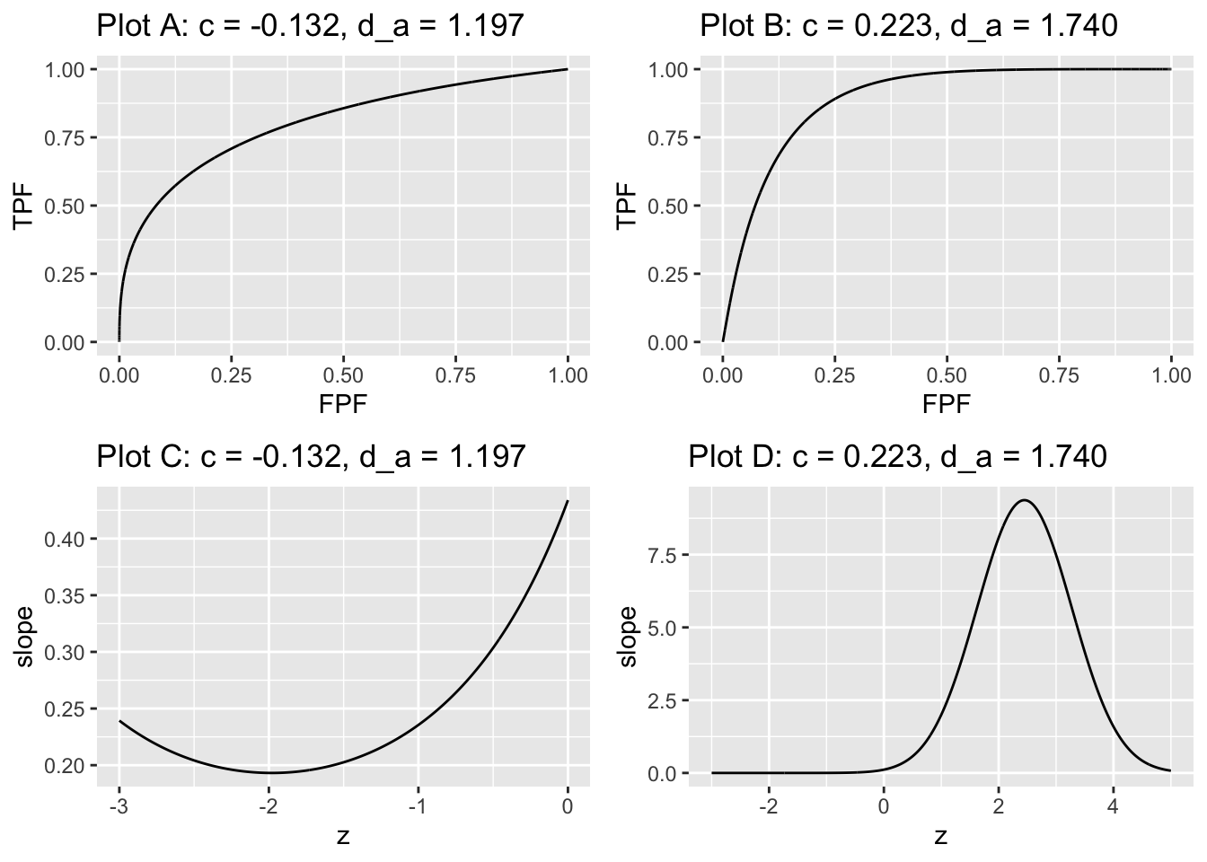
FIGURE 7.2: The plots are labeled by the values of \(c\) and \(d_a\). Plots A and B are proper ROC plots while plots C and D are the corresponding slope plots. In plot A the slope is infinite near the origin finite at the upper-right corner. In plot B the slope is finite near the origin and zero at the upper-right corner.
Plot A is for a negative value of \(c\) which implies \(b < 1\). The slope of the proper ROC is infinite near the origin, corresponding to the very large values of slope in plot C at large likelihood ratio threshold \(\lambda\)), and the slope approaches a non-zero value near the upper right corner of the ROC, corresponding to the non-zero minimum slope in plot C approached as one lowers the likelihood threshold \(\lambda\)).
Plot B is for a positive value of \(c\) which implies \(b > 1\). This time the slope of the ROC near the origin is large but finite, corresponding to the peak in plot D at intermediate likelihood threshold \(\lambda\), and the slope approaches zero near the upper right corner, corresponding to the zero minimum slope in Plot D approached as one lowers the likelihood threshold \(\lambda\) to zero.
To better understand the relation between the ROC plots and the slope plots one moves up the ROC curve by “slicing” the slope axis in plots C and D with a downward sliding horizontal cut, i.e., the threshold \(\lambda\) is being lowered starting with a high value. In plot A the slope of the ROC curve starts at the origin with an infinite value corresponding to large slope at the top-right corner in plot C. In plot B the slope of the ROC curve starts at the origin with a finite value corresponding to the finite peak in plot D. Above the peak, there are no solutions for \(z\). The slope decreases monotonically to zero corresponding to the flattening out of the slope at zero for \(z \approx 2\).
Alternatively, one can think of horizontally shrinking each of plots C and D to zero width, and all that remains is the slope axis with a thick vertical line superimposed on it corresponding to the horizontally collapsed curve. In plot C this vertical line extends from positive infinity down to about 0.1 and represents the range of decision variable samples encountered by the observer using the likelihood ratio scale. In plot D this vertical line extends from \(\approx 9.4\) to zero. Values outside of these ranges are not possible for the given parameter values of the underlying binormal model.
The two values of z that can occur for each value of \(\lambda\) implies that the binormal model based proper ROC algorithm has to do a lot of bookkeeping.
7.7 The contaminated binormal model (CBM)
The contaminated binormal model (Dorfman, Berbaum, and Brandser 2000; Dorfman and Berbaum 2000b, 2000a), or CBM, is an alternate model for decision variable sampling in an ROC study. Like the binormal model, it is a two-parameter model, excluding cutoffs. The first parameter is \(\mu_\text{CBM}\), the separation of two unit-variance normal distributions. The sampling for non-diseased cases is from the \(N(0,1)\) distribution, while sampling for diseased cases is from the \(N(\mu_\text{CBM},1)\) distribution, provided the disease is visible, otherwise it is from the \(N(0,1)\) distribution. In other words, for diseased cases the sampling is from a mixture distribution of two unit variance normal distributions, one centered at \(\mu\) and the other centered at 0, with mixing fraction \(\alpha\), the fraction of diseased cases where the abnormality is actually visible. The binning is accomplished, as usual, by the cutoff vector \(\overrightarrow{\zeta}=\left( \zeta_1,...,\zeta_{\text{ROC}-1} \right)\), where \(R_\text{ROC}\) is the number of ROC bins. Defining dummy cutoffs \(\zeta_0=-\infty\) and \(\zeta_{\text{ROC}}=\infty\), the binning rule is as before:
\[\begin{equation} \left.\begin{aligned} \text{if}~\left (\zeta_{r-1} \le z < \zeta_r \right ) \text{rating} = r\\ r=1,2,...,R_{ROC} \end{aligned}\right\} \tag{7.18} \end{equation}\]
Therefore, CBM is characterized by the parameters \(\mu, \alpha, \overrightarrow{\zeta}\). The parameters \(\mu, \alpha\) can be used to predict the ROC curve and the area under the curve.
7.7.1 CBM formulae
For non-diseased cases, the \(\text{pdf}\) is the same as for the binormal model:
\[\begin{equation} \text{pdf}_N=\phi(z) \tag{7.19} \end{equation}\]
For diseased cases the \(\text{pdf}\) is a mixture of two unit variance distributions, one centered at zero and the other at \(\mu_\text{CBM}\), with mixing fractions \((1-\alpha)\) and \(\alpha\), respectively:
\[\begin{equation} \text{pdf}_D=\left( 1-\alpha \right)\phi(z) + \alpha \phi(z-\mu_\text{CBM}) \tag{7.20} \end{equation}\]
The likelihood ratio for the CBM model is given by the ratio of the two pdfs:
\[\begin{equation} \left.\begin{aligned} l_\text{CBM}\left( z|a,b \right)&=\frac{\left( 1-\alpha \right)\phi(z) + \alpha \phi(z-\mu_\text{CBM})}{\phi(z)}\\ &=\left( 1-\alpha \right)+\alpha \, \exp\left(-\frac{\mu_\text{CBM}^2}{2}+z\,\mu_\text{CBM} \right) \end{aligned}\right\} \tag{7.21} \end{equation}\]
The function increases monotonically as \(z\) increases which shows that the predicted ROC curve is proper, i.e., its slope decreases monotonically as the operating point moves up the curve (causing both \(z\) and the likelihood ratio to decrease). The slope at the origin (infinite \(z\)) is infinite and the slope at the upper-right corner is \((1-\alpha)\). The predicted ROC coordinates are:
\[\begin{equation} \left.\begin{aligned} \text{FPF}\left( \zeta \right) &= \Phi\left( -\zeta \right)\\ \text{TPF}\left( \zeta \right) &= \left( 1-\alpha \right)\Phi\left( -\zeta \right)+\alpha \,\Phi\left( \mu_\text{CBM}-\zeta \right) \end{aligned}\right\} \tag{7.22} \end{equation}\]
Since on non-diseased cases the sampling behaviors are identical, the expression for \(\text{FPF}\left( \zeta \right)\) is identical to that for the binormal model: the probability that the z-sample for a non-diseased case exceeds \(\zeta\) is \(\Phi\left( -\zeta \right)\). The second Eqn. (7.22) can be understood as follows. \(\text{TPF}\left( \zeta \right)\) is the probability that a diseased case z-sample exceeds \(\zeta\). There are two possibilities: the z-sample arose from the zero-centered distribution, which occurs with probability \(\left( 1-\alpha \right)\), or it arose from the \(\mu_\text{CBM}\)-centered distribution, which occurs with probability \(\alpha\). In the former case, the probability that the z-sample exceeds \(\zeta\) is \(\Phi\left( -\zeta \right)\). In the latter case, the probability is \(\Phi\left( \mu_\text{CBM}-\zeta \right)\). The net probability is the weighted sum of the component probabilities in proportion to their relative frequencies \(\left( 1-\alpha \right):\alpha\).
A similar logic can be used to derive the AUC under the CBM fitted ROC curve:
\[\begin{equation} \text{AUC}_\text{CBM}=0.5\left( 1-\alpha \right)+\alpha \,\Phi\left( \frac {\mu_\text{CBM}}{\sqrt{2}} \right) \tag{7.23} \end{equation}\]
In the limit \(\mu_\text{CBM} \rightarrow \infty\), \(\text{AUC}_\text{CBM} \rightarrow 0.5\left( 1+\alpha \right)\) and in the limit \(\mu_\text{CBM} \rightarrow 0\), \(\text{AUC}_\text{CBM} \rightarrow 0.5\).
7.7.2 CBM ROC plots
The following figures should further clarify these equations. Fig. 7.3 shows ROC curves predicted by the CBM model; the values of the \(\alpha\) and \(\mu\) parameters are indicated in the legend. For small \(\alpha\) and/or small \(\mu\) the curve approaches the chance diagonal consistent with the notion that if the lesion is not visible performance can be no better than chance level.
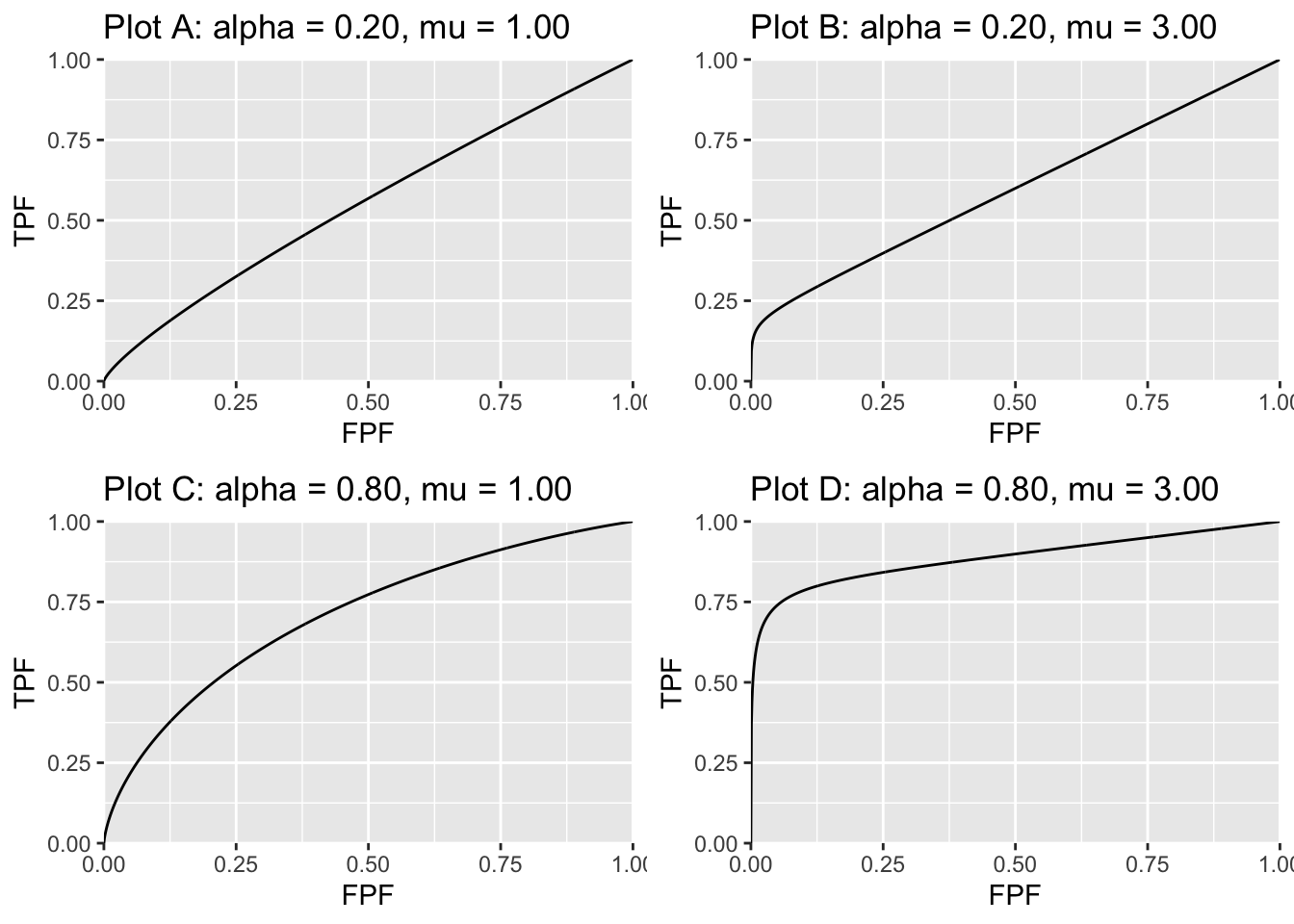
FIGURE 7.3: ROC curves predicted by the CBM model. The corresponding values of the parameters are indicated above the plots. For small \(\alpha\) or small \(\mu\) the curve approaches the chance diagonal, consistent with the notion that if the lesion is not visible, performance can be no better than chance level.
As one might expect as \(\mu\) and/or \(\alpha\) increases performance gets better and the curve more closely approaches the top-left corner. The predicted ROC curve is always proper.
The pdf plots are shown next, Fig. 7.4.
7.7.3 CBM pdf plots
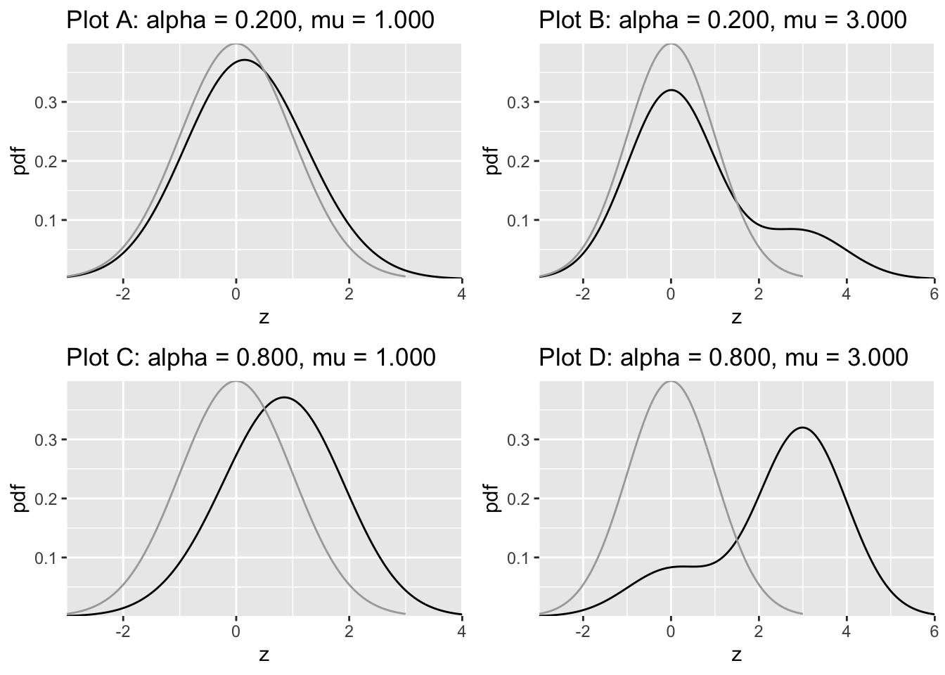
FIGURE 7.4: Density functions predicted by CBM. The dark line is the diseased distribution. The grey line is the non-diseased distribution. The bimodal diseased distribution is clearly evident in plots B and D.
Likelihood ratio plots are shown next, Fig. 7.5.
7.7.4 CBM likelihood ratio plots
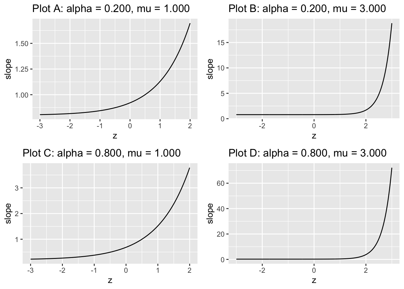
FIGURE 7.5: The slope plots are labeled by the values of \(\alpha\) and \(\mu\). Close examination of the region near the flat part shows it does not plateau at zero; rather the minimum is at \((1 - \alpha)\).
All plots are monotonic with \(z\): as \(z\) increases the slope increases. The reader using \(z\) to make decisions, where z is sampled as in the CBM model, is a likelihood ratio observer. In addition, according to TBA Eqn. (20.26), the limiting slope at the upper right corner of the ROC plot approaches \(1-\alpha\) as \(z \rightarrow –\infty\).
–>
7.8 Discussion
With the readily availability of CBM and RSM (both implemented in RJafroc) there is no excuse for not using them. These programs are indeed “bullet-proof”: they can fit any dataset that one cares to throw at them. The author’s preference is to use RSM as it yields additional information about search and lesion-localization performance not available using CBM. PROPOROC has some problems fitting degenerate datasets that can be readily fixed but to my knowledge no one is actively maintaining this important contribution by Prof. Metz.
7.9 Appendix: Metz Eqn 36 numerical check
The \(c\) and \(d_a\) parameters used here are from an FROC study in breast tomosynthesis (Andersson et al. 2008). There are two modalities and five readers.
7.9.1 Main code and output
#>    i j           c        da aucProproc     normDiff
#> 1  1 1 -0.13228036 1.1972393  0.8014164 3.520017e-08
#> 2  1 2 -0.08696513 1.7711756  0.8947898 4.741875e-08
#> 3  1 3 -0.14444185 1.4819349  0.8526605 3.515431e-08
#> 4  1 4  0.08046016 1.5137569  0.8577776 4.971428e-08
#> 5  1 5  0.22255876 1.7401572  0.8909392 2.699855e-08
#> 6  2 1 -0.08174248 0.6281251  0.6716574 2.801793e-08
#> 7  2 2  0.04976448 0.9738786  0.7544739 5.275242e-08
#> 8  2 3 -0.13261262 1.1558707  0.7931787 3.472577e-08
#> 9  2 4  0.11822263 1.6201757  0.8740274 3.922161e-08
#> 10 2 5  0.07810330 0.8928816  0.7360989 3.798459e-08
Note the close correspondence between the formula, Eqn. 36 in (Charles E. Metz and Pan 1999), and the numerical estimate. Eqn. 31 and Eqn. 36 in the paper (they differ only in parameterizations) are provided without proof – it was probably obvious to Prof Metz or he wanted to leave it to us “mere mortals” to figure it out as a final parting gesture of his legacy. The author once put a significant effort into proving it and even had a bright graduate student from the biostatistics department work on it to no avail. I have observed that these equations always yield very close to the numerical estimates so the theorem is obviously empirically correct, but I have been unable to prove it analytically.