Chapter 10 Bivariate models
10.2 Introduction
Until now the focus of this book has been on the single rating per case scenario where a reader interprets a set of cases in a single modality. This chapter describes two approaches to the problem of two readers interpreting a common set of cases. The first approach extends the binormal model to paired interpretations while the second extends the contaminated binormal model to paired interpretations. The corresponding software implementations are CORROC2 (for correlated ROC) and CORCBM (for correlated CBM), respectively (because of the paired interpretation the two ratings per case are correlated).
In my book (Dev P. Chakraborty 2017) Chapter 21 was devoted to the CORROC2 algorithm and usage of the software was described in some detail. At that time (Zhai and Chakraborty 2017) was in press. It describes an alternate algorithm that has several advantages over CORROC2. Therefore, I have reconsidered the focus of this chapter which now outlines the correlated binormal model fitting procedure but does not detail how to use CORROC2 software. Instead I now include the work presented in (Zhai and Chakraborty 2017) including interactive 3D visualization of the distributions which is not possible in print. The abbreviated description showing how to extend the binormal model to a correlated binormal model, described in the first section, will help the reader better understand how to extend the contaminated binormal model to the correlated contaminated binormal model, described in the second section.
10.3 The bivariate binormal model
Described next is the bivariate normal distribution followed by its extension to the bivariate binormal distribution.
10.3.1 The bivariate normal distribution
Sampling from the bivariate normal distribution \(N_2\) is as follows:
\[\begin{equation} \overrightarrow{z} \sim N_2\left( \overrightarrow{\mu}, \Sigma \right) \tag{10.1} \end{equation}\]
Here \(\overrightarrow{z}\) is a length-\(2\) vector, with components \((z_1,z_2)\), of the observed z-samples for each case, \(\overrightarrow{\mu}\) is a length-\(2\) vector containing the means of the bivariate normal distribution and \(\Sigma\) is a \(2 \times 2\) covariance matrix describing the variances and correlations of the observed z-samples.
The bivariate normal probability density function \(\text{pdf}\left( \overrightarrow{z} ~~ \bigg \rvert ~~\overrightarrow{\mu}, ~~ \Sigma \right)\) is defined by:
\[\begin{equation} \text{pdf}\left( z_1,z_2 ~~ \bigg \rvert ~~ \overrightarrow{\mu}, \Sigma \right) = \frac{1}{2 \pi \sigma_1 \sigma_2 \sqrt{1-\rho^2}}\exp\left( -\frac{t}{2\left( 1-\rho^2 \right)} \right) \tag{10.2} \end{equation}\]
where
\[\begin{equation} t=\frac{\left( z_1-\mu_1 \right)^2}{\sigma_1^2}-\frac{2\rho\left( z_1-\mu_1 \right)\left( z_2-\mu_2 \right)}{\sigma_1 \sigma_2} +\frac{\left( z_2-\mu_2 \right)^2}{\sigma_2^2} \tag{10.3} \end{equation}\]
For a bivariate distribution the covariance matrix is:
\[\begin{equation} \Sigma= \left( \begin{matrix} \sigma_1^2 & \rho \sigma_1 \sigma_2 \\ \rho \sigma_1 \sigma_2 & \sigma_2^2 \end{matrix} \right)\tag{10.4} \end{equation}\]
In these equations \(\mu_1\) and \(\sigma_1^2\) is the mean and variance for modality 1, \(\mu_2\) and \(\sigma_2^2\) is the mean and variance for modality 2 and \(\rho\) is the correlation between the two modalities.
The R function to evaluate Eqn. (10.2) is dmvnorm(), for “density of multivariate normal distribution”, available via package mvtnorm (Genz et al. 2023). Its usage is illustrated next for the following parameter values:
\[\begin{equation} \left.\begin{aligned} \overrightarrow{ \mu}&= \left( \begin{matrix} \mu_1 \\ \mu_2 \end{matrix} \right) =\left( \begin{matrix} 1.5 \\ 2.0 \end{matrix} \right) \\ \sigma_1 &= 1.1 \\ \sigma_2 &= 1.5 \\ \rho &= 0.6 \\ \Sigma&= \left( \begin{matrix} \sigma_1^2 & \rho \sigma_1 \sigma_2 \\ \rho \sigma_1 \sigma_2 & \sigma_2^2 \end{matrix}\right) = \left( \begin{matrix} 1.1^2 & 0.6 \times 1.1 \times 1.5 \\ 0.6 \times 1.1 \times 1.5 & 1.5^2 \end{matrix}\right)\end{aligned}\right\} \tag{10.5} \end{equation}\]
In the following code the call to get the pdf occurs at line 10.
mu1 <- 1.5 # mean modality 1
mu2 <- 2.0 # mean modality 2
var1 <- 1.1^2  # variance modality 1
var2 <- 1.5^2 # variance modality 2
rho <- 0.6 # correlation between modalities 1 and 2
# construct covariance matrix Sigma
Sigma <- matrix(c(var1, rho*sqrt(var1*var2),
                  rho*sqrt(var1*var2), var2),2)
x <- c(0.1,0.2) # the x-vector at which to evaluate pdf
pdf  <- dmvnorm(x, mean = c(mu1,mu2), sigma = Sigma)
cat("density at x1 = 0.1 and x2 = 0.2 = ", pdf, "\n")
#> density at x1 = 0.1 and x2 = 0.2 =  0.04622722
The parameters describing the bivariate normal distribution are \(\overrightarrow{\mu}\) and \(\Sigma\). The total number of parameters is five: two means, two variances and a correlation coefficient.
10.3.2 The bivariate binormal model
The bivariate binormal model is an extension of the bivariate model just described to two truth-states: non-diseased and diseased, each modeled separately and independently as a bivariate normal distribution. This could potentially result in a doubling of the number of parameters but by appropriate shifting and scale transformations one can ensure that the two means of the bivariate distribution for non-diseased cases are zeroes and the corresponding variances are unity. This reduces the total number of parameters to six: \(\mu_{12}\), \(\mu_{22}\), \(\sigma_{12}\), \(\sigma_{22}\), \(\rho_1\), \(\rho_2\). Here \(\mu_{12}\), \(\mu_{22}\) are the means for diseased cases for modality 1 and modality 2, respectively, \(\sigma_{12}^2\), \(\sigma_{22}^2\) are the corresponding variances and \(\rho_1\), \(\rho_2\) are the correlations between the two modalities for non-diseased and diseased cases, respectively.
Notation: henceforth when there are two subscripts the first subscript refers to the modality and the second to the truth state. When there is only one subscript it refers to the truth state.
The bivariate binormal parameters are:
\[\begin{equation} \left.\begin{aligned} \overrightarrow{ \mu_1}&= \left( \begin{matrix} 0 \\ 0 \end{matrix} \right)\\ \overrightarrow{ \mu_2}&= \left( \begin{matrix} \mu_{12} \\ \mu_{22} \end{matrix} \right)\\ \Sigma_1&= \left( \begin{matrix} 1 & \rho_1 \\ \rho_1 & 1 \end{matrix} \right) \\ \Sigma_2 &= \left( \begin{matrix} \sigma_{12}^2 & \rho_2 \sigma_{12} \sigma_{22} \\ \rho_2 \sigma_{12} \sigma_{22} & \sigma_{22}^2 \end{matrix} \right) \end{aligned}\right\} \tag{10.6} \end{equation}\]
The decision variable is \(z_{ik_tt}\) where the \(i\) subscript corresponds to the two modalities and the \(t\) subscript corresponds to the two truth states. The paired-ratings \(\left( z_{1k_11},z_{2k_11} \right)\) and \(\left( z_{1k_22},z_{2k_22} \right)\), corresponding to z-samples from non-diseased and diseased cases, respectively, are abbreviated to \(\overrightarrow{z_{1k_tt}}\) (the vectorization always “condenses” the two modalities):
\[\begin{equation} \overrightarrow{z_{k_tt}}= \left( \begin{matrix} z_{1k_tt} \\ z_{2k_tt} \end{matrix} \right) \tag{10.7} \end{equation}\]
\(\overrightarrow{z_{k_tt}}\) is sampled as follows:
\[\begin{equation} \overrightarrow{z_{k_tt}} \sim N_2\left( \overrightarrow{\mu_t}, \Sigma_t \right) \tag{10.8} \end{equation}\]
The parameters \(\overrightarrow{\mu_t}, \Sigma_t\) are truth-state dependent as described in Eqn. (10.6).
To complete the model one needs to include threshold parameters and a decision rule. Recall that for an R-rating single modality ROC task with allowed ratings \(r = 1, 2, ..., \text{R}\), one needs \(\text{R}-1\) thresholds \(\zeta_1,\zeta_2,...,\zeta_{\text{R}-1}\). Defining \(\zeta_0 = -\infty\) and \(\zeta_{\text{R}} = +\infty\) the decision rule is to label a case with rating \(r\) if the realized z-sample satisfies \(\zeta_{r-1} < z \le \zeta_r\).
In the two-modality task the decision variable and the thresholds are modality dependent: i.e., \(z_{1k_tt}\) and \(z_{2k_tt}\) and two sets of thresholds are needed: \(\overrightarrow{\zeta_1} \equiv \zeta_{11},\zeta_{12},...,\zeta_{1 (\text{R}-1)}\) and \(\overrightarrow{\zeta_2} \equiv\zeta_{21},\zeta_{22},...,\zeta_{2 (\text{S}-1)}\), where \(R\) is the number of allowed ratings in modality 1 and \(S\) is the number of allowed ratings in modality 2 (they can be different). As before \(\zeta_{10} = -\infty\) and \(\zeta_{20} = -\infty\) and \(\zeta_{1\text{R}} = +\infty\) and \(\zeta_{2\text{S}} = +\infty\). The decision rule is to rate a case in modality \(1\) with rating \(r\) if \(\zeta_{1(r-1)} < z_{1k_tt} \le \zeta_{1r}\) and the same case in modality \(2\) is rated \(s\) if \(\zeta_{2(s-1)} < z_{2k_tt} \le \zeta_{2s}\).
10.3.3 Visualizing the bivariate binormal density functions
It is helpful to visualize the pdfs. One needs two axes to depict the two z-samples and a third to depict the pdf. This is done for non-diseased cases in Fig. 10.1, and for diseased cases in Fig. 10.2. The plots are interactive and the reader may wish to experiment by clicking and dragging the cursor on them. Package plotly (Sievert et al. 2024) provides the visualization technique.
The parameters are as follows:
FIGURE 10.1: Interactive plot of the bivariate binormal pdf function for non-diseased cases for \(\rho_1 = 0.3\). The peak is at (0,0) and each marginal distributions has unit variance. Modality 1 is plotted along x and modality 2 along y.
FIGURE 10.2: Interactive plot of the bivariate binormal pdf function for diseased cases for \(\rho_2 = 0.6\). The peak is at (1.5, 2.0) and the marginal distributions for modality 1 has standard deviation 1.1 and that for modality 2 has standard deviation 1.5.
10.3.4 Estimating bivariate binormal model parameters
Chapter 6 described a method for estimating the parameters of the univariate binormal model. It involved maximizing the likelihood function, i.e., the probability of the observed data as a function of the model parameters. The values of the parameters at the maximum are the maximum-likelihood estimates (MLEs).
With a bivariate model one is dealing with six non-threshold parameters \(\overrightarrow{\mu_t}, \Sigma_t\) plus threshold parameters for each modality. Again, the starting point is the likelihood function. The non-diseased case counts in bin \(r\) of the first modality and bin \(s\) of the second modality is denoted by \(K_{rs1}\) (i.e., the binning indices occur before the truth index). The corresponding diseased counts are denoted \(K_{rs2}\). Each case yields two integer ratings, \(r\) and \(s\).
For non-diseased cases, the probability \(p_{rs1}\) of a z-sample in bin \(r\) of the first modality and bin \(s\) of the second modality is determined by the “volume” under the bivariate distribution \(N_2(\overrightarrow {\mu_1}, \Sigma_1)\) between modality-1 thresholds \(\zeta_{1(r-1)}\) and \(\zeta_{1r}\), and between modality-2 thresholds \(\zeta_{2(s-1)}\) and \(\zeta_{2s}\). For diseased cases the corresponding probability \(p_{rs2}\) is the volume under the bivariate distribution \(N_2(\overrightarrow {\mu_2}, \Sigma_2)\) between the same thresholds. These probabilities can be calculated using the pmvnorm() function in package (Genz et al. 2023).
The probability of observing \(K_{rs1}\) non-diseased cases and \(K_{rs2}\) diseased cases in bin \(r\) in the first modality and bin \(s\) in the second modality is:
\[\begin{equation} \prod_{t=1}^{2}\left ( p_{rst} \right )^{K_{rst}} \end{equation}\]
The logarithm of the likelihood function is given by (neglecting a combinatorial factor that does not depend on the parameters):
\[\begin{equation} LL\left ( \overrightarrow{\mu_2}, \Sigma_1, \Sigma_2, \overrightarrow{\zeta_1},\overrightarrow{\zeta_2} \right ) = \sum_{t=1}^{2}\sum_{s=1}^{S}\sum_{r=1}^{R} K_{rst} \log(p_{rst}) \end{equation}\]
The MLEs of the parameters are obtained by maximizing the LL function, (Charles E. Metz and Kronman 1980; Charles E. Metz, Wang, and Kronman 1984), implemented in CORROC2. A unique feature is that the software measures ratings-correlations at the underlying z-sample level. Much as I have emphasized that ratings are not “hard” numbers the CORROC2 estimated correlations are valid because the algorithm models the ratings as continuous variables and estimates the correlation based on the bivariate binormal model.
10.4 The bivariate contaminated binormal model
The bivariate contaminated binormal model (BCBM) is the bivariate extension of the univariate contaminated binormal model described in Chapter 7. Corresponding to the two truth states the BCBM is defined by two bivariate distributions as described next.
10.4.1 Non-diseased cases
For non-diseased cases the sampling is as follows:
\[\begin{equation} \overrightarrow{z_{k_11}} \sim N_2\left( \overrightarrow{\mu_1}, \Sigma_1 \right) \tag{10.10} \end{equation}\]
where
\[\begin{equation} \left.\begin{aligned} \overrightarrow{ \mu_1}&= \left( \begin{matrix} 0 \\ 0 \end{matrix} \right)\\ \Sigma_1&= \left( \begin{matrix} 1 & \rho_1 \\ \rho_1 & 1 \end{matrix} \right) \\ \end{aligned}\right\} \tag{10.11} \end{equation}\]
10.4.2 Diseased cases
Recall, Eqn. (7.20), that in the (univariate) CBM, for diseased cases the pdf is a mixture of two scaled unit variance distributions, one centered at zero and the other at \(\mu\) that integrate (i.e., via the scale factors) to \((1-\alpha)\) and \(\alpha\), respectively.
The extension to bivariate sampling needs to account for the possibility that the scale factors can be different in the two modalities, modeled by \(\alpha_1\) and \(\alpha_2\), and the z-sample means for cases where the disease is visible can be different in the two modalities, modeled by \(\mu_{12}\) and \(\mu_{22}\) and finally one must account for four possibilities described next:
The disease is not visible in either modality. The appropriate distribution is a scaled bivariate \(N_2\) distribution centered at \(\overrightarrow{\mu_{00}} \equiv (0,0)\) with correlation \(\rho_{00}\) whose pdf integrates to \((1-\alpha_1)(1-\alpha_2)\).
The disease is visible in modality 1 but not visible in modality 2. The appropriate distribution is a scaled bivariate \(N_2\) distribution centered at \(\overrightarrow{\mu_{10}} \equiv (\mu_{12},0)\) with correlation \(\rho_{10}\) whose pdf integrates to \(\alpha_1(1-\alpha_2)\).
The disease is not visible in modality 1 but is visible in modality 2. The appropriate distribution is a scaled bivariate \(N_2\) distribution centered at \(\overrightarrow{\mu_{01}} \equiv (0,\mu_{22})\) with correlation \(\rho_{01}\) whose pdf integrates to \((1-\alpha_1)\alpha_2\).
The disease is visible in both modalities 1 and 2. The appropriate distribution is a scaled bivariate \(N_2\) distribution centered at \(\overrightarrow{\mu_{11}} \equiv (\mu_{12},\mu_{22})\) with correlation \(\rho_{11}\) whose pdf integrates to \(\alpha_1\alpha_2\).
The means and covariance matrices for the four distributions are defined by:
\[\begin{equation} \left.\begin{aligned} \begin{matrix} \overrightarrow{ \mu_{00}}&= \left( \begin{matrix} 0 \\ 0 \end{matrix} \right) & \Sigma_{00}&= \left( \begin{matrix} 1 & \rho_{00} \\ \rho_{00} & 1 \end{matrix} \right) \\ \\ \overrightarrow{ \mu_{10}}&= \left( \begin{matrix} \mu_{12} \\ 0 \end{matrix} \right) & \Sigma_{10}&= \left( \begin{matrix} 1 & \rho_{10} \\ \rho_{10} & 1 \end{matrix} \right) \\ \\ \overrightarrow{ \mu_{01}}&= \left( \begin{matrix} 0 \\ \mu_{22} \end{matrix} \right) & \Sigma_{01}&= \left( \begin{matrix} 1 & \rho_{01} \\ \rho_{01} & 1 \end{matrix} \right) \\ \\ \overrightarrow{ \mu_{11}}&= \left( \begin{matrix} \mu_{12} \\ \mu_{22} \end{matrix} \right) & \Sigma_{11}&= \left( \begin{matrix} 1 & \rho_{11} \\ \rho_{11} & 1 \end{matrix} \right) \\ \end{matrix} \end{aligned}\right\} \tag{10.12} \end{equation}\]
Therefore, the pdf of the diseased case bivariate distribution is:
\[\begin{equation} \left.\begin{aligned} \text{pdf}\left (z_{1k_22},z_{2k_22} \right ) = &(1-\alpha_1)(1-\alpha_2)~~\text{pdf}\left ( z_{1k_22},z_{2k_22} ~| ~\overrightarrow{\mu_{00}}, \Sigma_{00}\right )\\ +& \alpha_1(1-\alpha_2)~~\text{pdf}\left ( z_{1k_22},z_{2k_22} ~| ~ \overrightarrow{\mu_{10}}, \Sigma_{10}\right )\\ +& (1-\alpha_1)\alpha_2~~\text{pdf}\left ( z_{1k_22},z_{2k_22} ~| ~ \overrightarrow{\mu_{01}}, \Sigma_{01}\right )\\ +& \alpha_1\alpha_2~~\text{pdf}\left ( z_{1k_22},z_{2k_22} ~| ~\overrightarrow{\mu_{11}}, \Sigma_{11}\right )\\ \end{aligned}\right\} \tag{10.13} \end{equation}\]
In this equation \(\text{pdf}\left ( z_{1k_22},z_{2k_22} ~| ~\overrightarrow{\mu}, \Sigma \right )\) denotes the bivariate normal pdf function with the specified mean-vector and covariance matrix, as defined in Eqn. (10.2).
3D interactive visualization plots that follow are for the following parameters:
FIGURE 10.3: Interactive surface plot showing the 4 distributions that are needed to describe diseased case sampling.
Fig. 10.3 this pdf function is shown as a surface plot and four peaks are visible.
(Zhai and Chakraborty 2017) prove that with the above scale factors the pdf and CDF (cumulative distribution function) of the marginal distributions for diseased cases in modalities 1 and 2 have the same structure as in the univariate CBM, i.e., either condition, viewed in isolation, has the same sampling behavior as the univariate CBM.
The above model has four correlations in contrast to the bivariate binormal model which has two correlations. For parsimony the following assumptions are made:
When the disease is invisible in both modalities the correlation is the same as that for non-diseased cases, i.e., \(\rho_{00} \equiv \rho_1\).
When the disease is visible in both modalities the correlation is \(\rho_{11} \equiv \rho_2\).
When the disease is visible in only one modality the correlation is the mean of the non-diseased cases correlation and the correlation where disease is visible in both conditions, i.e., \(\rho_{10} = \rho_{01} = (\rho_1+\rho_2)/2\).
10.4.3 Estimation
This follows the procedure described previously for the correlated binormal model (i.e., CORROC2). One introduces binning thresholds, defines the likelihood function and applies a procedure for maximizing it. Details are in (Zhai and Chakraborty 2017) which also shows applications to two real datasets and a simulation study.
10.4.4 Application to Van Dyke dataset
Fig. 10.4; CORCBM fits for Van Dyke data for reader 4. CORROC2 failed to converge.
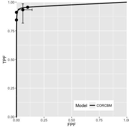
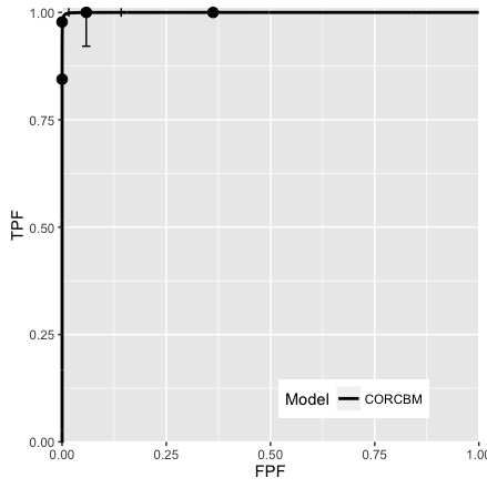
FIGURE 10.4: VanDyke dataset, reader 4. Left plot: modality 1, right plot: modality 2. CORROC2 failed to converge and therefore only CORCBM plots are shown.
Fig. 10.5; CORROC2 (dashed line) and CORCBM (solid line) fits for Van Dyke data for reader 5.
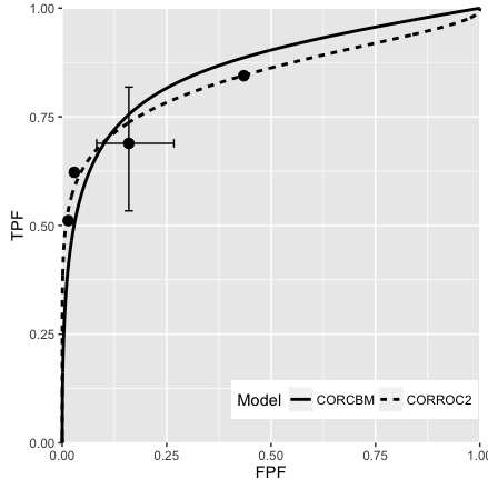
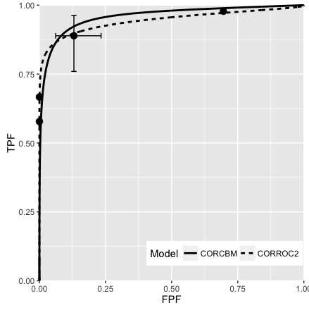
FIGURE 10.5: VanDyke dataset, reader 5. Left plot: modality 1, right plot: modality 2; both CORROC2 (dashed line) and CORCBM (solid line) plots are shown. Note that CORCBM has higher AUC than CORROC2.
10.4.5 Simulation study
Fig. 10.6; simulation parameters were \(\mu_1 = 1.5\), \(\mu_2 = 3\), \(\alpha_1 = 0.4\), \(\alpha_2 = 0.7\), \(\rho_1 = 0.3\), \(\rho_2 = 0.8\).
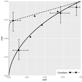
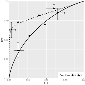
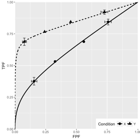
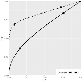
FIGURE 10.6: CORCBM fits to simulated data for two modalities labeled “conditions”. Top-left: 50 non-diseased and 50 diseased cases; Top-right: 100 non-diseased and 100 diseased cases; Bottom-left: 1000 non-diseased and 1000 diseased cases; Bottom-right: 5000 non-diseased and 5000 diseased cases. For 5000-5000 cases the operating points are almost exactly fitted by CORCBM.
10.5 Discussion
Described is an approach to fitting paired ROC datasets using a bivariate extension of the contaminated binormal model. Software implementing the method, CORCBM, was applied to two datasets that have been widely used to test methodological advances in ROC analysis. For comparison CORROC2, which implements the bivariate binormal model, was also applied to the same datasets. CORCBM was able to fit the paired data for all 9 readers (5 from the Van Dyke dataset and 4 from the Franken dataset) while CORROC2 was unable to fit one reader in the Van Dyke dataset. Inability to fit a dataset, especially for a reader whose performance is close to perfect is, in my opinion, a serious shortcoming. (Vannier et al. 1994) have reported a study where CORROC2 was unable to fit 14 out of 16 clinical datasets. All CORROC2 fits are improper implying a range of predicted performance that is below the chance diagonal for expert radiologists, another serious shortcoming.
In our opinion extending PROPROC, a relatively complex algorithm, whose software is not in the public domain, to paired data would be a challenge. Moreover, since it is based on the binormal model, it would still be unable to yield reasonable fits to degenerate datasets. The authors have confirmed that given a dataset with 100 non-diseased and 100 diseased cases yielding a single operating point at (0, TPF), where 0 < TPF < 1, PROPROC yields AUC = 1 regardless of how small the value of TPF is, which is unreasonable. Likewise, given a dataset yielding a single operating point at (FPF, 0), where 0 < FPF < 1, PROPROC still yields AUC = 1 regardless of how large the value of FPF is, which is also unreasonable. The CBM model is simpler and has no issues with fitting degenerate datasets. In my opinion, the CBM model parameters are easier to interpret than other proper ROC models, and as shown in this work, it can be extended to the bivariate situation.
Our interest in this problem arose from a methodology validation issue. Multiple-reader multiple case (MRMC) study designs are widely used to compare modalities and several analysis methods have been proposed. The Dorfman Berbaum Metz method or the substantially equivalent Obuchowski and Rockette method have been used in a few hundred publications (Prof. Kevin Berbaum, private communication, ca. 2010). With such wide usage the results of any of which could be a critical driver of medical imaging technology, one needs to be sure that the analysis method is valid. Validating a methodology requires an MRMC ratings data simulator. The simulator used so far to validate DBM is that proposed by Roe and Metz. This simulator has several shortcomings. It assumes that the ratings are distributed like an equal-variance binormal model, which is not true for most clinical datasets. CBM provides a natural explanation of the observed unequal variance: since there are two types of disease – visible and not visible –the mixing of the two gives arise to a diseased case pdf that appears wider than a non-diseased case pdf. The Roe-Metz simulator is out dated: the parameter values are based on datasets then available (i.e., prior to 1997). Medical imaging technology has changed substantially in the intervening decades, and modalities that did not exist then, like digital mammography, breast and chest tomosynthesis, are in wide usage in the US. Finally, the method used to arrive at the Roe and Metz parameter values is not clearly described. Needed is a realistic simulator that is calibrated by a clearly defined method to current datasets.
My approach to this problem originally used CORROC2 to determine the different types of ratings-level correlations present in an ROC-MRMC dataset. The correlations were used to design a simulator that incorporated the measured values. However, CORROC2 frequently failed to converge in many instances and other discrepancies were found when CORROC2 was applied to newer datasets (CORROC2 gave reasonable results for the Van Dyke and the Franken datasets, but failed to converge on almost all newer datasets). This is what led to this work.
An application of CORCBM to calibrating a simulator to a clinical data set is described in the next Chapter TBA 23.
10.3.5 Comments on CORROC2
CORROC2 was developed as described in (Charles E. Metz, Wang, and Kronman 1984). Subsequent revisions to the program were made by Jong-Her Shen and more recently by Benjamin Herman (C. Metz et al. 1989; Charles E. Metz, Herman, and Roe 1998). There are at least 116 citations to this software. One reason is that at the time (mid 1980s) it was the only software that allowed significance testing of paired single-reader datasets. However, no advances have been made in the intervening 3 decades, which would allow fitting proper ROC curves to paired datasets. There has been a shift to empirical AUC based analysis which does not require parametric modeling. CORROC2 is currently a relatively under-utilized tool. One reason is that it is not designed to analyze multiple readers interpreting a common set of cases in two or more modalities i.e., MRMC datasets, which is of current interest. The main weakness of CORROC2 is its dependence on the underlying binormal model which, as we have seen, is susceptible to improper ROC curves and degeneracy problems.