Chapter 3 FROC data format
3.2 Introduction
The purpose of this chapter is to explain the format of the FROC Excel file and how to read this file into a dataset object suitable for analysis using the RJafroc package.
In the FROC paradigm the observer assigns a rating and a location to suspicious regions in images that exceed the reporting threshold. As an example a CAD algorithm may find tens of suspicious regions in each image but the algorithm designer only shows those regions (typically one or two) whose confidence levels exceed the chosen threshold.
The chapter is illustrated with a toy data file, R/quick-start/frocCr.xlsx in which readers ‘0’, ‘1’ and ‘2’ interpret 8 cases in two modalities, ‘0’ and ‘1’. The design is ‘factorial’, abbreviated to FCTRL in the software; this is also termed a ‘fully-crossed’ design. The Excel file has three worksheets named Truth, NL (or FP) and LL (or TP). These names are case-insensitive.
3.3 The Truth worksheet
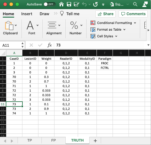
The Truth worksheet contains 6 columns: CaseID, LesionID, Weight, ReaderID, ModalityID and Paradigm. Since a diseased case may have more than one lesion, the first five columns contain at least as many rows as there are cases in the dataset. There are 8 cases (‘1’,‘2’,‘3’,‘70’,‘71’,‘72’,‘73’ and ‘74’) in the dataset and 12 rows in the Truth worksheet, because some of the diseased cases contain more than one lesion.
CaseID: unique integers representing the individual cases in the dataset: e.g., ‘1’, ‘2’, ‘3’, the 3 non-diseased cases and ‘70’, ‘71’, ‘72’, ‘73’, ‘74’, the 5 diseased cases. The ordering of the numbers is inconsequential. 2LesionID: non-negative integers 0, 1, 2, …, where:- Each 0 represents a non-diseased case, e.g., this field is zero for non-diseased cases ‘1’, ‘2’ and ‘3’.
- Each 1 represents the first lesion in a diseased case, 2 represents the second lesion, if present, and so on.
Weightor clinical importance associated with lesion:- It is 0 for each non-diseased case,
- For each diseased case the values must sum to unity.
- A shortcut to assigning equal weights to all lesions in a case is to fill the
Weightcolumn with zeroes.
ReaderID: see Section 2.5.1.ModalityID: see Section 2.5.1.Paradigm: see Section 2.5.1.
3.3.1 Comments on the Truth worksheet
There are 3 non-diseased cases in the dataset (the number of 0’s in the LesionID column). There are 5 diseased cases in the dataset (the number of 1’s in the LesionID column). There are 3 readers in the dataset labeled ‘0, 1, 2’. There are 2 modalities in the dataset labeled ‘0, 1’. Diseased case 70 has two lesions, with LesionIDs ‘1’ and ‘2’ and weights 0.3 and 0.7, respectively. Diseased case 71 has one lesion with LesionID = 1 and Weight = 1. Diseased case 72 has three lesions with LesionIDs 1, 2 and 3 and weights 1/3 each. Diseased case 73 has two lesions, with LesionIDs 1, and 2 and weights 0.1 and 0.9, respectively. Diseased case 74 has one lesion, with LesionID = 1 and Weight = 1. Note that LesionIDs identify the lesions - for example, a lesion with high morbidity may be labeled LesionID = 1 and assigned weight 0.9 while a second lower morbidity lesion on the same case may be assigned LesionID = 2 and weight 0.1. In this example reversing the lesion IDs would lead to incorrect weight assignments.
3.4 The FP ratings
These are found in the FP or NL worksheet.
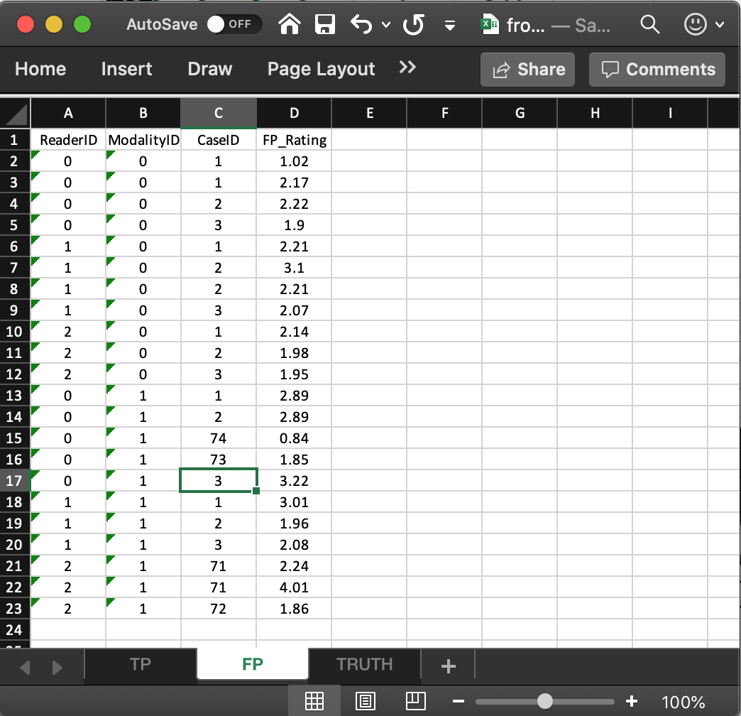
It consists of 4 columns of equal length. The common length is an integer random variable \(\ge 0\). It could be zero if the dataset has no NL marks (a possibility if the lesions are easy to find or the observer has perfect performance). In this example the common length is 22, which is a-priori unpredictable: for example, if the dataset has many FPs it could be large.
ReaderID: the reader labels: these must be one of0,1, or2as declared in theTruthworksheet.ModalityID: the modality labels: must be one of0or1as declared in theTruthworksheet.CaseID: the labels of cases withNLmarks. These must be one of1,2,3,70,71,72,73,74as declared in theTruthworksheet. In the FROC paradigmNLevents can occur on non-diseased and diseased cases.FP_Rating: the floating point ratings ofNLmarks. Each cell contains the rating corresponding to the values ofReaderID,ModalityIDandCaseIDfor that row.
3.4.1 Comments on the FP worksheet
For
ModalityID0,ReaderID0 andCaseID1 (the first non-diseased case declared in theTruthworksheet), there is a singleNLmark that was rated 1.02, corresponding to row 2 of theFPworksheet.Diseased cases with
NLmarks are also recorded in theFPworksheet. Some examples are seen at rows 15, 16 and 21, 22, 23. Rows 21 and 22 show thatcaseID= 71 got twoNLmarks, rated 2.24, 4.01.Since this is the only case with two NL marks, it determines the length of the fourth dimension of the
ds$ratings$NL, which is 2 in this example. Absent this case, the length would have been one. The case with the mostNLmarks determines the length of the fourth dimension ofds$ratings$NL. The reader should confirm that the ratings inds$ratings$NLreflect the contents of theFPworksheet.
3.5 The TP ratings
These are found in the TP or LL worksheet, see below.
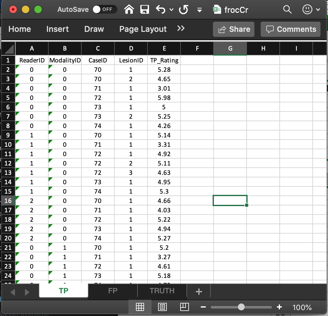
This worksheet can only have diseased cases. The presence of a non-diseased case will generate an error. The common vertical length, 31 in this example, is a-priori unpredictable (as some lesions may not be marked). The maximum possible length, assuming every lesion is marked for each modality, reader and diseased case, is 9 X 2 X 3 = 54. The 9 comes from the total number of non-zero entries in the LesionID column of the Truth worksheet, the 2 from the number of modalities and 3 from the number of readers.
The fact that the actual length (31) is smaller than the maximum length (54) means that there are combinations of modality, reader and diseased cases on which some lesions were not marked.
As examples, line 2 in the worksheet, the first lesion in CaseID equal to 70 was marked (and rated 5.28) in ModalityID 0 and ReaderID 0. Line 3 in the worksheet, the second lesion in CaseID equal to 70 was also marked (and rated 4.65) in ModalityID 0 and ReaderID 0. However, lesions 2 and 3 in CaseID = 72 were not marked (line 5 in the worksheet indicates that for this modality-reader-case combination only the first lesion was marked). The reader should confirm that the ratings in ds$ratings$LL reflect the contents of the TP worksheet.
3.6 Reading the FROC dataset
The example shown above corresponds to file R/quick-start/frocCr.xlsx in the project directory. The next code reads this file into an R object ds.
frocCr <- "R/quick-start/frocCr.xlsx"
ds <- DfReadDataFile(frocCr, newExcelFileFormat = TRUE)
str(ds)
#> List of 3
#>  $ ratings     :List of 3
#>   ..$ NL   : num [1:2, 1:3, 1:8, 1:2] 1.02 2.89 2.21 3.01 2.14 ...
#>   ..$ LL   : num [1:2, 1:3, 1:5, 1:3] 5.28 5.2 5.14 4.77 4.66 4.87 3.01 3.27 3.31 3.19 ...
#>   ..$ LL_IL: logi NA
#>  $ lesions     :List of 3
#>   ..$ perCase: int [1:5] 2 1 3 2 1
#>   ..$ IDs    : num [1:5, 1:3] 1 1 1 1 1 ...
#>   ..$ weights: num [1:5, 1:3] 0.3 1 0.333 0.1 1 ...
#>  $ descriptions:List of 7
#>   ..$ fileName     : chr "frocCr"
#>   ..$ type         : chr "FROC"
#>   ..$ name         : logi NA
#>   ..$ truthTableStr: num [1:2, 1:3, 1:8, 1:4] 1 1 1 1 1 1 1 1 1 1 ...
#>   ..$ design       : chr "FCTRL"
#>   ..$ modalityID   : Named chr [1:2] "0" "1"
#>   .. ..- attr(*, "names")= chr [1:2] "0" "1"
#>   ..$ readerID     : Named chr [1:3] "0" "1" "2"
#>   .. ..- attr(*, "names")= chr [1:3] "0" "1" "2"
This follows the general description in Chapter 2. The differences are described below.
The
ds$descriptions$typemember indicates that this is anFROCdataset.The
ds$lesions$perCasemember is a vector containing the number of lesions in each diseased case, i.e., 2, 1, 3, 2, 1 in the current example.The
ds$lesions$IDsmember indicates the labeling of the lesions in each diseased case.
ds$lesions$IDs
#>      [,1] [,2] [,3]
#> [1,]    1    2 -Inf
#> [2,]    1 -Inf -Inf
#> [3,]    1    2    3
#> [4,]    1    2 -Inf
#> [5,]    1 -Inf -Inf
This shows that the lesions on the first diseased case are labeled ‘1’ and ‘2’. The
-Infis a filler denoting a missing value. The second diseased case has one lesion labeled ‘1’. The third diseased case has three lesions labeled ‘1’, ‘2’ and ‘3’, etc.The
lesionWeightmember is the clinical importance of each lesion. Lacking specific clinical reasons, the lesions should be equally weighted; this is not true for this toy dataset (except for the third diseased case).
ds$lesions$weights
#>           [,1]      [,2]      [,3]
#> [1,] 0.3000000 0.7000000      -Inf
#> [2,] 1.0000000      -Inf      -Inf
#> [3,] 0.3333333 0.3333333 0.3333333
#> [4,] 0.1000000 0.9000000      -Inf
#> [5,] 1.0000000      -Inf      -Inf
The first diseased case has two lesions, the first has weight 0.3 and the second has weight 0.7.
The second diseased case has one lesion with weight 1.
The third diseased case has three equally weighted lesions, each with weight 1/3. Etc.
3.7 The distribution of lesions in diseased cases
Consider a much larger real dataset, dataset11, with structure as shown below (for descriptions of all embedded datasets see Chapter 12):
ds <- dataset11
str(ds)
#> List of 3
#>  $ ratings     :List of 3
#>   ..$ NL   : num [1:4, 1:5, 1:158, 1:4] -Inf -Inf -Inf -Inf -Inf ...
#>   ..$ LL   : num [1:4, 1:5, 1:115, 1:20] -Inf -Inf -Inf -Inf -Inf ...
#>   ..$ LL_IL: logi NA
#>  $ lesions     :List of 3
#>   ..$ perCase: int [1:115] 6 4 7 1 3 3 3 8 11 2 ...
#>   ..$ IDs    : num [1:115, 1:20] 1 1 1 1 1 1 1 1 1 1 ...
#>   ..$ weights: num [1:115, 1:20] 0.167 0.25 0.143 1 0.333 ...
#>  $ descriptions:List of 7
#>   ..$ fileName     : chr "dataset11"
#>   ..$ type         : chr "FROC"
#>   ..$ name         : chr "DOBBINS-1"
#>   ..$ truthTableStr: num [1:4, 1:5, 1:158, 1:21] 1 1 1 1 1 1 1 1 1 1 ...
#>   ..$ design       : chr "FCTRL"
#>   ..$ modalityID   : Named chr [1:4] "1" "2" "3" "4"
#>   .. ..- attr(*, "names")= chr [1:4] "1" "2" "3" "4"
#>   ..$ readerID     : Named chr [1:5] "1" "2" "3" "4" ...
#>   .. ..- attr(*, "names")= chr [1:5] "1" "2" "3" "4" ...
The large number of lesions is explained by the fact that this is a volumetric CT image for lung nodule detection (each nodule was verified by 3 radiologists).
Focus on the 115 diseased cases: the numbers of lesions in individual cases is contained in ds$lesions$perCase.
ds$lesions$perCase
#>   [1]  6  4  7  1  3  3  3  8 11  2  4  6  2 16  5  2  8  3  4  7 11  1  4  3  4
#>  [26]  4  7  3  2  5  2  2  7  6  6  4 10 20 12  6  4  7 12  5  1  1  5  1  2  8
#>  [51]  3  1  2  2  3  2  8 16 10  1  2  2  6  3  2  2  4  6 10 11  1  2  6  2  4
#>  [76]  5  2  9  6  6  8  3  8  7  1  1  6  3  2  1  9  8  8  2  2 12  1  1  1  1
#> [101]  1  3  1  2  2  1  1  1  1  3  1  1  1  2  1
For example, the first diseased case contains 6 lesions, the second contains 4 lesions, the third contains 7 lesions, etc., and the last diseased case contains 1 lesion. To get the distribution of the numbers of lesions per diseased cases one could use the which() function:
for (el in 1:max(ds$lesions$perCase)) cat(
  "number of diseased cases with", el, "lesions = ",
  length(which(ds$lesions$perCase == el)), "\n")
#> number of diseased cases with 1 lesions =  25
#> number of diseased cases with 2 lesions =  23
#> number of diseased cases with 3 lesions =  13
#> number of diseased cases with 4 lesions =  10
#> number of diseased cases with 5 lesions =  5
#> number of diseased cases with 6 lesions =  11
#> number of diseased cases with 7 lesions =  6
#> number of diseased cases with 8 lesions =  8
#> number of diseased cases with 9 lesions =  2
#> number of diseased cases with 10 lesions =  3
#> number of diseased cases with 11 lesions =  3
#> number of diseased cases with 12 lesions =  3
#> number of diseased cases with 13 lesions =  0
#> number of diseased cases with 14 lesions =  0
#> number of diseased cases with 15 lesions =  0
#> number of diseased cases with 16 lesions =  2
#> number of diseased cases with 17 lesions =  0
#> number of diseased cases with 18 lesions =  0
#> number of diseased cases with 19 lesions =  0
#> number of diseased cases with 20 lesions =  1
This tells us that 25 cases contain 1 lesion. Likewise, 23 cases contain 2 lesions, etc. Note that there are no cases with 13, 14, 15, 17, 18, and 19 lesions.
3.7.1 Definition of lesID array
The fraction of diseased cases with 1 lesion, 2 lesions etc, can be calculated as follows:
for (el in 1:max(ds$lesions$perCase))
  cat("fraction of diseased cases with", el, "lesions = ",
  length(which(ds$lesions$perCase == el))/length(ds$ratings$LL[1,1,,1]), "\n")
#> fraction of diseased cases with 1 lesions =  0.2173913
#> fraction of diseased cases with 2 lesions =  0.2
#> fraction of diseased cases with 3 lesions =  0.1130435
#> fraction of diseased cases with 4 lesions =  0.08695652
#> fraction of diseased cases with 5 lesions =  0.04347826
#> fraction of diseased cases with 6 lesions =  0.09565217
#> fraction of diseased cases with 7 lesions =  0.05217391
#> fraction of diseased cases with 8 lesions =  0.06956522
#> fraction of diseased cases with 9 lesions =  0.0173913
#> fraction of diseased cases with 10 lesions =  0.02608696
#> fraction of diseased cases with 11 lesions =  0.02608696
#> fraction of diseased cases with 12 lesions =  0.02608696
#> fraction of diseased cases with 13 lesions =  0
#> fraction of diseased cases with 14 lesions =  0
#> fraction of diseased cases with 15 lesions =  0
#> fraction of diseased cases with 16 lesions =  0.0173913
#> fraction of diseased cases with 17 lesions =  0
#> fraction of diseased cases with 18 lesions =  0
#> fraction of diseased cases with 19 lesions =  0
#> fraction of diseased cases with 20 lesions =  0.008695652
Fraction 0.217 of diseased cases contain 1 lesion, fraction 0.2 of (diseased) cases contain 2 lesions, etc.
This information is more readily obtained using the RJafroc function UtilLesDistr() as shown next (be sure to view both screens):
UtilLesDistr(ds)
#>    lesID        Freq
#> 1      1 0.217391304
#> 2      2 0.200000000
#> 3      3 0.113043478
#> 4      4 0.086956522
#> 5      5 0.043478261
#> 6      6 0.095652174
#> 7      7 0.052173913
#> 8      8 0.069565217
#> 9      9 0.017391304
#> 10    10 0.026086957
#> 11    11 0.026086957
#> 12    12 0.026086957
#> 13    13 0.000000000
#> 14    14 0.000000000
#> 15    15 0.000000000
#> 16    16 0.017391304
#> 17    17 0.000000000
#> 18    18 0.000000000
#> 19    19 0.000000000
#> 20 20 0.008695652- The
UtilLesDistr()function returns a dataframe with two columns. - The first column (
lesID) contains the number of lesions per case. - The second column (
Freq) contains the fraction of diseased cases with the number of lesions indicated in the first column. - The second column sums to unity:
sum(UtilLesDistr(ds)$Freq)
#> [1] 1
3.8 Lesion weights
- This
dataframeis returned byUtilLesWghtsDS()orUtilLesWghtsLD(). - This contains the same number of rows as
lesID. - The number of columns is one plus the number of rows.
- The first column contains the number of lesions per case.
- The second through the last column contain the weights of cases with number of lesions per case in column 1.
- Missing values are filled with
-Inf.
UtilLesWghtsDS(ds, relWeights = 0)
#>       [,1]       [,2]       [,3]       [,4]       [,5]       [,6]       [,7]
#>  [1,]    1 1.00000000       -Inf       -Inf       -Inf       -Inf       -Inf
#>  [2,]    2 0.50000000 0.50000000       -Inf       -Inf       -Inf       -Inf
#>  [3,]    3 0.33333333 0.33333333 0.33333333       -Inf       -Inf       -Inf
#>  [4,]    4 0.25000000 0.25000000 0.25000000 0.25000000       -Inf       -Inf
#>  [5,]    5 0.20000000 0.20000000 0.20000000 0.20000000 0.20000000       -Inf
#>  [6,]    6 0.16666667 0.16666667 0.16666667 0.16666667 0.16666667 0.16666667
#>  [7,]    7 0.14285714 0.14285714 0.14285714 0.14285714 0.14285714 0.14285714
#>  [8,]    8 0.12500000 0.12500000 0.12500000 0.12500000 0.12500000 0.12500000
#>  [9,]    9 0.11111111 0.11111111 0.11111111 0.11111111 0.11111111 0.11111111
#> [10,]   10 0.10000000 0.10000000 0.10000000 0.10000000 0.10000000 0.10000000
#> [11,]   11 0.09090909 0.09090909 0.09090909 0.09090909 0.09090909 0.09090909
#> [12,]   12 0.08333333 0.08333333 0.08333333 0.08333333 0.08333333 0.08333333
#> [13,]   13 0.07692308 0.07692308 0.07692308 0.07692308 0.07692308 0.07692308
#> [14,]   14 0.07142857 0.07142857 0.07142857 0.07142857 0.07142857 0.07142857
#> [15,]   15 0.06666667 0.06666667 0.06666667 0.06666667 0.06666667 0.06666667
#> [16,]   16 0.06250000 0.06250000 0.06250000 0.06250000 0.06250000 0.06250000
#> [17,]   17 0.05882353 0.05882353 0.05882353 0.05882353 0.05882353 0.05882353
#> [18,]   18 0.05555556 0.05555556 0.05555556 0.05555556 0.05555556 0.05555556
#> [19,]   19 0.05263158 0.05263158 0.05263158 0.05263158 0.05263158 0.05263158
#> [20,]   20 0.05000000 0.05000000 0.05000000 0.05000000 0.05000000 0.05000000
#>             [,8]       [,9]      [,10]      [,11]      [,12]      [,13]
#>  [1,]       -Inf       -Inf       -Inf       -Inf       -Inf       -Inf
#>  [2,]       -Inf       -Inf       -Inf       -Inf       -Inf       -Inf
#>  [3,]       -Inf       -Inf       -Inf       -Inf       -Inf       -Inf
#>  [4,]       -Inf       -Inf       -Inf       -Inf       -Inf       -Inf
#>  [5,]       -Inf       -Inf       -Inf       -Inf       -Inf       -Inf
#>  [6,]       -Inf       -Inf       -Inf       -Inf       -Inf       -Inf
#>  [7,] 0.14285714       -Inf       -Inf       -Inf       -Inf       -Inf
#>  [8,] 0.12500000 0.12500000       -Inf       -Inf       -Inf       -Inf
#>  [9,] 0.11111111 0.11111111 0.11111111       -Inf       -Inf       -Inf
#> [10,] 0.10000000 0.10000000 0.10000000 0.10000000       -Inf       -Inf
#> [11,] 0.09090909 0.09090909 0.09090909 0.09090909 0.09090909       -Inf
#> [12,] 0.08333333 0.08333333 0.08333333 0.08333333 0.08333333 0.08333333
#> [13,] 0.07692308 0.07692308 0.07692308 0.07692308 0.07692308 0.07692308
#> [14,] 0.07142857 0.07142857 0.07142857 0.07142857 0.07142857 0.07142857
#> [15,] 0.06666667 0.06666667 0.06666667 0.06666667 0.06666667 0.06666667
#> [16,] 0.06250000 0.06250000 0.06250000 0.06250000 0.06250000 0.06250000
#> [17,] 0.05882353 0.05882353 0.05882353 0.05882353 0.05882353 0.05882353
#> [18,] 0.05555556 0.05555556 0.05555556 0.05555556 0.05555556 0.05555556
#> [19,] 0.05263158 0.05263158 0.05263158 0.05263158 0.05263158 0.05263158
#> [20,] 0.05000000 0.05000000 0.05000000 0.05000000 0.05000000 0.05000000
#>            [,14]      [,15]      [,16]      [,17]      [,18]      [,19]
#>  [1,]       -Inf       -Inf       -Inf       -Inf       -Inf       -Inf
#>  [2,]       -Inf       -Inf       -Inf       -Inf       -Inf       -Inf
#>  [3,]       -Inf       -Inf       -Inf       -Inf       -Inf       -Inf
#>  [4,]       -Inf       -Inf       -Inf       -Inf       -Inf       -Inf
#>  [5,]       -Inf       -Inf       -Inf       -Inf       -Inf       -Inf
#>  [6,]       -Inf       -Inf       -Inf       -Inf       -Inf       -Inf
#>  [7,]       -Inf       -Inf       -Inf       -Inf       -Inf       -Inf
#>  [8,]       -Inf       -Inf       -Inf       -Inf       -Inf       -Inf
#>  [9,]       -Inf       -Inf       -Inf       -Inf       -Inf       -Inf
#> [10,]       -Inf       -Inf       -Inf       -Inf       -Inf       -Inf
#> [11,]       -Inf       -Inf       -Inf       -Inf       -Inf       -Inf
#> [12,]       -Inf       -Inf       -Inf       -Inf       -Inf       -Inf
#> [13,] 0.07692308       -Inf       -Inf       -Inf       -Inf       -Inf
#> [14,] 0.07142857 0.07142857       -Inf       -Inf       -Inf       -Inf
#> [15,] 0.06666667 0.06666667 0.06666667       -Inf       -Inf       -Inf
#> [16,] 0.06250000 0.06250000 0.06250000 0.06250000       -Inf       -Inf
#> [17,] 0.05882353 0.05882353 0.05882353 0.05882353 0.05882353       -Inf
#> [18,] 0.05555556 0.05555556 0.05555556 0.05555556 0.05555556 0.05555556
#> [19,] 0.05263158 0.05263158 0.05263158 0.05263158 0.05263158 0.05263158
#> [20,] 0.05000000 0.05000000 0.05000000 0.05000000 0.05000000 0.05000000
#>            [,20] [,21]
#>  [1,]       -Inf  -Inf
#>  [2,]       -Inf  -Inf
#>  [3,]       -Inf  -Inf
#>  [4,]       -Inf  -Inf
#>  [5,]       -Inf  -Inf
#>  [6,]       -Inf  -Inf
#>  [7,]       -Inf  -Inf
#>  [8,]       -Inf  -Inf
#>  [9,]       -Inf  -Inf
#> [10,]       -Inf  -Inf
#> [11,]       -Inf  -Inf
#> [12,]       -Inf  -Inf
#> [13,]       -Inf  -Inf
#> [14,]       -Inf  -Inf
#> [15,]       -Inf  -Inf
#> [16,]       -Inf  -Inf
#> [17,]       -Inf  -Inf
#> [18,]       -Inf  -Inf
#> [19,] 0.05263158  -Inf
#> [20,] 0.05000000  0.05
## or
## UtilLesWghtsLD(UtilLesDistr(ds), relWeights = 0)
##- Row 3 corresponds to 3 lesions per case and the weights are 1/3, 1/3 and 1/3.
- Row 13 corresponds to 13 lesions per case and the weights are 0.06250000, 0.06250000, …, repeated 13 times.
- Note that the number of rows equals the maximum number of lesions per case (20).
CaseIDshould not be so large that it cannot be represented in Excel by an integer; to be safe use unsigned short 8-bit integers.↩︎