Chapter 10 FROC sample size estimation

10.1 How much finished 99 percent

10.2 Overview

This chapter is split into two parts:

Part 1 is a step-by-step (or first-principles) approach to FROC paradigm sample size estimation.
Part 2 encapsulates some of the details in function SsFrocNhRsmModel() which makes it easier to use the sample size estimation method.

10.3 Part 1

10.3.1 Introduction

FROC sample size estimation is not fundamentally different from ROC sample size estimation detailed in Chapter 8 and summarized next.

Summary of ROC sample size estimation

Based on analysis of a pilot ROC dataset and using a specified figure of merit (FOM), e.g., FOM = Wilcoxon, and either method = "DBM" or method = "OR" for significance testing, one estimates the intrinsic variability of the data expressed in terms of FOM variance components. For the DBM method these are the pseudovalue-based variance components while for OR method these are the FOM-based variance and covariances. In this chapter the OR method will be used. The second step is to specify a clinically realistic effect-size, e.g., the anticipated AUC difference between the two modalities.

Given the variance components and the anticipated AUC difference the sample size functions (RJafroc function names beginning with Ss) allow one to estimate the number of readers and cases necessary to detect (i.e., reject the null hypothesis) the modality AUC difference with probability $\beta$, typically chosen to be 20 percent (corresponding to 80 percent statistical power) while maintaining the NH (zero AUC difference) rejection rate probability at $\alpha$, typically chosen to be 5 percent.

Summary of FROC sample size estimation

In FROC analysis the only difference, indeed the critical difference, is the choice of FOM; e.g., FOM = "wAFROC" instead of the ROC-AUC, FOM = "Wilcoxon". The FROC dataset is analyzed using the OR method. This yields the covariance matrix corresponding to wAFROC-AUC FOM. Next one specifies the effect-size in wAFROC-AUC units and this step requires care. The ROC-AUC has a historically well-known interpretation, namely it is the classification ability at separating diseased patients from non-diseased patients, while the wAFROC-AUC does not. Needed is a way of relating the effect-size in the easily understood ROC-AUC unit to one in wAFROC-AUC unit. This requires a physical model, e.g., the RSM, that predicts both ROC and wAFROC curves and their corresponding AUCs.

One chooses an ROC-AUC effect-size that is realistic and one that clinicians understand and can therefore participate in the effect-size postulation process. Lacking such information I recommend, based on past ROC studies, 0.03 as typical of a small effect size and 0.05 as typical of a moderate effect size.
One converts the ROC effect-size to a wAFROC-AUC effect-size using the method described in the next section.
One uses the sample size tools in RJafroc to determine sample size for a desired statistical power.

It is important to recognize is that all quantities have to be in the same units. When performing ROC analysis, everything (variance components and effect-size) has to be in units of the selected FOM, e.g., FOM = "Wilcoxon". When performing wAFROC analysis, everything has to be in units of the wAFROC-AUC, i.e., FOM = "wAFROC". The variance components and effect-size in wAFROC-AUC units will be different from their corresponding ROC counterparts. In particular, as shown next, a given ROC-AUC effect-size generally corresponds to a larger effect-size in wAFROC-AUC units. The reason for this is that the range over which wAFROC-AUC can vary, namely 0 to 1, which is twice the corresponding ROC-AUC range (0.5 to 1). For the same reason the wAFROC variance components also tend to be larger than the ROC variance components.

The next section explains the steps used to implement #2 above.

10.3.2 Relating ROC and wAFROC effect-sizes

The steps are illustrated using dataset04, a 5 treatment, 4 radiologist and 200 case FROC dataset (Zanca et al. 2009) acquired on a 5-point scale.

10.3.2.1 Extract NH treatments

If there are more than two treatments in the pilot dataset, as in dataset04, one extracts those treatments that represent “almost” null hypothesis data (in the sense of similar AUCs):

frocDataNH <- DfExtractDataset(dataset04, trts = c(1,2))

The preceding code extracts treatments 1 and 2 which were found (Zanca et al. 2009) to be “almost” equivalent (i.e., the NH could not be rejected for the wAFROC-AUC difference between these treatments). More than two almost NH treatments can be used if they have similar AUCs, as this will improve the stability of the procedure. However, the final sample size predictions are restricted to two treatments in the pivotal study.

The next two steps are needed since the RSM fits binned ROC data.

10.3.2.2 Convert the FROC NH data to ROC

If the original data is FROC one converts it to ROC:

rocDataNH <- DfFroc2Roc(frocDataNH)

10.3.2.3 Bin the data

If the NH dataset uses continuous ratings one bins the ratings:

# For dataset04 this is unnecessary as it is already binned, but it can't hurt, i.e.,
# rocDataBinNH <- rocDataNH # gives same results as following line
rocDataBinNH <- DfBinDataset(rocDataNH, opChType = "ROC")

The default number of bins should be used. Unlike binning using arbitrarily set thresholds the thresholds found by DfBinDataset() are unique as they are chosen to maximize the empirical ROC-AUC.

10.3.2.4 Determine the lesion distribution and weights of the FROC dataset

lesDistr is the lesion distribution, see Section 3.7.1 and line 1 of the following code. The RSM fitting algorithm needs to know how lesion-rich the dataset is as the predicted ROC-AUC depends on it. For this dataset fraction 0.69 of diseased cases have one lesion, fraction 0.2 have two lesions and fraction 0.11 have three lesions. One also needs the lesion weights matrix, $\textbf{W}$, see Section 3.8. The call at line 2 to UtilLesWghtsDS uses the default argument relWeights = 0 which assigns equal weights to all lesions.

lesDistr <- UtilLesDistr(frocDataNH)
W <- UtilLesWghtsDS(frocDataNH)

Note that lesDistr and $\textbf{W}$ are determined from the FROC NH dataset as this information is lost upon conversion to an ROC dataset.

10.3.2.5 Fit the RSM to the ROC data

For each treatment and reader the fitting algorithm FitRsmRoc() is applied (see below, lines 4 - 11) to the binned NH ROC dataset. The returned values are mu, lambda and nu, corresponding to the physical RSM parameters $\mu$, $\lambda$ and $\nu$.

I <- dim(rocDataBinNH$ratings$NL)[1] # number of levels of treatment factor
J <- dim(rocDataBinNH$ratings$NL)[2] # number of levels of reader factor
RsmParmsNH <- array(dim = c(I,J,3)) # 3 corresponds to the three RSM parameters
for (i in 1:I) {
  for (j in 1:J)  {
    fit <- FitRsmRoc(rocDataBinNH, trt = i, rdr = j, lesDistr$Freq)
    RsmParmsNH[i,j,1] <- fit[[1]] # mu
    RsmParmsNH[i,j,2] <- fit[[2]] # lambda
    RsmParmsNH[i,j,3] <- fit[[3]] # nu
  }
}

10.3.2.6 Compute the median values of the RSM parameters

I recommend taking the median (not the mean) of the $I \times J$ values of each parameter as representing the average NH dataset (he median is less sensitive to outliers than the mean).

muNH <- median(RsmParmsNH[,,1]) 
lambdaNH <- median(RsmParmsNH[,,2])
nuNH <- median(RsmParmsNH[,,3])

The defining values of the RSM-based NH fitting model are muNH = 3.3121491, lambdaNH = 1.714368 and nuNH = 0.7036564.

10.3.2.7 Compute ROC and wAFROC NH AUCs

The next step is the compute the analytical (i.e., RSM-based) AUCs under the respective ROC and the wAFROC curves:

aucRocNH <- UtilAnalyticalAucsRSM(muNH, lambdaNH, nuNH, lesDistr = lesDistr$Freq)$aucROC
aucwAfrocNH <- UtilAnalyticalAucsRSM(muNH, lambdaNH, nuNH, lesDistr = lesDistr$Freq)$aucwAFROC

The AUCs are: aucRocNH = 0.8791541 and aucwAfrocNH = 0.7198614. Note that the wAFROC-FOM is smaller than the ROC-FOM as it includes both detection and localization performance (the ROC-AUC only measures detection performance).

10.3.2.8 Compute ROC and wAFROC Alternative Hypotheses AUCs for a range of ROC-AUC effect sizes

To create the alternative hypothesis (AH) condition, one increments $\mu_{NH}$ by $\Delta\mu$. Tempting as it may be, it is not enough to simply increase the $\mu$ parameter as increasing $\mu$ will simultaneously decrease $\lambda$ and increase $\nu$ (see the Astronomical Analogy in the RJafrocFrocBook). To account for this tandem effect one extracts the intrinsic parameters $\lambda_i, \nu_i$, at line 7 of the following code, and then converts back to the physical parameters at line 9 using the incremented $\mu$. Note the usage of the functions Util2Intrinsic (convert physical to intrinsic) and Util2Physical (convert intrinsic to physical) . The resulting ROC-AUC and wAFROC-AUC are then calculated. This yields the effect size (AH value minus NH value) using ROC and wAFROC FOMs for a series of specified $\Delta\mu$ values. These are used to relate the wAFROC effect size for a specified ROC effect size.

deltaMu <- seq(0.01, 0.2, 0.01)
esROC <- array(dim = length(deltaMu))
eswAFROC <- array(dim = length(deltaMu))

# get intrinsic parameters
par_i <- Util2Intrinsic(muNH, lambdaNH, nuNH) # convert physical to intrinsic

for (i in 1:length(deltaMu)) {
  
  # find physical parameters for the increased muNH (accounting for the tandem effects)
  par_p <- Util2Physical(muNH + deltaMu[i], par_i$lambda_i, par_i$nu_i)  # convert intrinsic to physical
  
  # AH ROC value minus NH ROC value
  esROC[i] <- UtilAnalyticalAucsRSM(
    muNH + deltaMu[i], par_p$lambda, par_p$nu, lesDistr = lesDistr$Freq)$aucROC - aucRocNH 
  
  # AH wAFROC value minus NH wAFROC value
  eswAFROC[i] <- UtilAnalyticalAucsRSM(
    muNH + deltaMu[i], par_p$lambda, par_p$nu, lesDistr = lesDistr$Freq)$aucwAFROC - aucwAfrocNH 
  
}

Here is a plot of wAFROC effect size (y-axis) vs. ROC effect size.

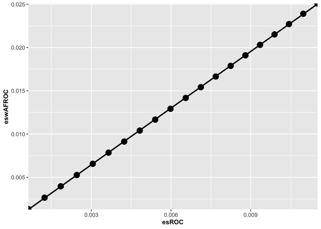
FIGURE 10.1: Plot of wAFROC effect size vs. ROC effect size. The straight line fit through the origin has slope 2.169.

The plot is linear and the intercept is close to zero. This makes it easy to implement an interpolation function. In the following code line 1 fits eswAFROC vs. esROC using a linear model lm() function constrained to pass through the origin (the “-1”). One expects this constraint since for deltaMu = 0 the effect size must be zero no matter how it is measured.

lmFit <- lm(eswAFROC ~ -1 + esROC) # the "-1" fits to straight line through the origin
scaleFactor <- lmFit$coefficients
effectSizeROC <- seq(0.01, 0.0525, 0.0025) 
effectSizewAFROC <- effectSizeROC*scaleFactor

The slope of the zero-intercept constrained straight line fit is scaleFactor = 2.169 and the squared correlation coefficient is R2 = 0.9999904 (the fit is very good). Therefore, the conversion from ROC to wAFROC effect size is:

effectSizewAFROC = scaleFactor * effectSizeROC

For this dataset the wAFROC effect size is 2.169 times the ROC effect size. The wAFROC effect size is expected to be larger than the ROC effect size because the range of wAFROC-AUC, $1-0=1$, is twice that of ROC-AUC, $1-0.5=0.5$.

10.3.3 ROC and wAFROC variance components

The following skeleton code shows the arguments of the function UtilORVarComp used to calculate the OR variance components (other arguments are left at their default values).

UtilORVarComp(
  dataset,
  FOM
)

UtilORVarComp() is applied to rocDataNH and frocDataNH (using “Wilcoxon” and “wAFROC” FOMs as appropriate) followed by the extraction of the ROC and wAFROC variance components.

varComp_roc <- UtilORVarComp(
  rocDataNH, 
  FOM = "Wilcoxon")$VarCom[-2]

varComp_wafroc <- UtilORVarComp(
  frocDataNH, 
  FOM = "wAFROC")$VarCom[-2]

VarCom[-2] removes the second column of each dataframe containing the correlations. The ROC and wAFROC variance components are:

##                ROC        wAFROC
## VarR  0.0008277380  0.0018542289
## VarTR 0.0001526507 -0.0004439279
## Cov1  0.0002083377  0.0003736844
## Cov2  0.0002388384  0.0003567162
## Cov3  0.0001906167  0.0003058902
## Var   0.0007307912  0.0009081383

10.3.4 ROC and wAFROC power for equivalent effect-sizes

The following code compares ROC and wAFROC random-reader random-case (RRRC) powers for equivalent effect sizes.

First, one needs the numbers of readers JStar and cases KStar in the pilot dataset (lines 1 - 2 in following code) and those in the pivotal study, JPivot and KPivot (line 3). The values for the pivotal study have been arbitrarily set at 5 readers and 100 cases.

JStar <- length(dataset04$ratings$NL[1,,1,1])
KStar <- length(dataset04$ratings$NL[1,1,,1])
JPivot <- 5;KPivot <- 100

Next one extracts the OR ROC variance components from the previously computed list varComp_roc.

# these are OR variance components assuming FOM = "Wilcoxon"
varR_roc <- varComp_roc["VarR","Estimates"]
varTR_roc <- varComp_roc["VarTR","Estimates"]
Cov1_roc <- varComp_roc["Cov1","Estimates"]
Cov2_roc <- varComp_roc["Cov2","Estimates"]
Cov3_roc <- varComp_roc["Cov3","Estimates"]
Var_roc <- varComp_roc["Var","Estimates"]

The procedure is repeated for the OR wAFROC variance components using the previously computed list varComp_wafroc.

# these are OR variance components assuming FOM = "wAFROC"
varR_wafroc <- varComp_wafroc["VarR","Estimates"]
varTR_wafroc <- varComp_wafroc["VarTR","Estimates"]
Cov1_wafroc <- varComp_wafroc["Cov1","Estimates"]
Cov2_wafroc <- varComp_wafroc["Cov2","Estimates"]
Cov3_wafroc <- varComp_wafroc["Cov3","Estimates"]
Var_wafroc <- varComp_wafroc["Var","Estimates"]

We are now ready for the power calculations. The needed function is SsPowerGivenJK (“sample size for given number of readers J and cases K”):

SsPowerGivenJK(
  dataset,
  FOM,
  J,
  K,
  effectSize,
  ...
)

In the following code the OR ROC variance components are passed to SsPowerGivenJK at lines 12-18. The OR wAFROC variance components are passed to SsPowerGivenJK at lines 29-34. Setting dataset = NULL means that the function does not need a dataset as the variance components are supplied instead using the ... argument.

The for-loop (lines 3 - 36) calculates ROC power (line 19) and wAFROC power (line 35) for a number of ROC (line 11) and corresponding wAFROC (line 28) effect sizes.

power_roc <- array(dim = length(effectSizeROC))
power_wafroc <- array(dim = length(effectSizeROC))
for (i in 1:length(effectSizeROC)) {
  # compute ROC power
  # dataset = NULL means use the supplied variance components instead of dataset
  ret <- SsPowerGivenJK(
    dataset = NULL, 
    FOM = "Wilcoxon", 
    J = JPivot, 
    K = KPivot, 
    effectSize = effectSizeROC[i], 
    list(JStar = JStar, 
         KStar = KStar, 
         VarTR = varTR_roc,
         Cov1 = Cov1_roc,
         Cov2 = Cov2_roc,
         Cov3 = Cov3_roc,
         Var = Var_roc))
  power_roc[i] <- ret$powerRRRC
  
  # compute wAFROC power
  # dataset = NULL means use the supplied variance components instead of dataset
  ret <- SsPowerGivenJK(
    dataset = NULL, 
    FOM = "wAFROC", 
    J = JPivot, 
    K = KPivot, 
    effectSize = effectSizewAFROC[i], 
    list(JStar = JStar, 
         KStar = KStar, 
         VarTR = varTR_wafroc,
         Cov1 = Cov1_wafroc,
         Cov2 = Cov2_wafroc,
         Cov3 = Cov3_wafroc,
         Var = Var_wafroc))
  power_wafroc[i] <- ret$powerRRRC
}

Since the wAFROC effect size is 2.169337 times the ROC effect size, wAFROC power is larger than ROC power. For example, for ROC effect size = 0.035 the wAFROC effect size is 0.076, the ROC power is 0.234 while the wAFROC power is 0.797. The influence of the increased wAFROC effect size is magnified as it enters as the square in the formula for statistical power: this overwhelms the increase, noted previously, in variability of wAFROC-AUC relative to ROC-AUC

The following is a plot of wAFROC power vs. ROC power for the specified effect sizes.

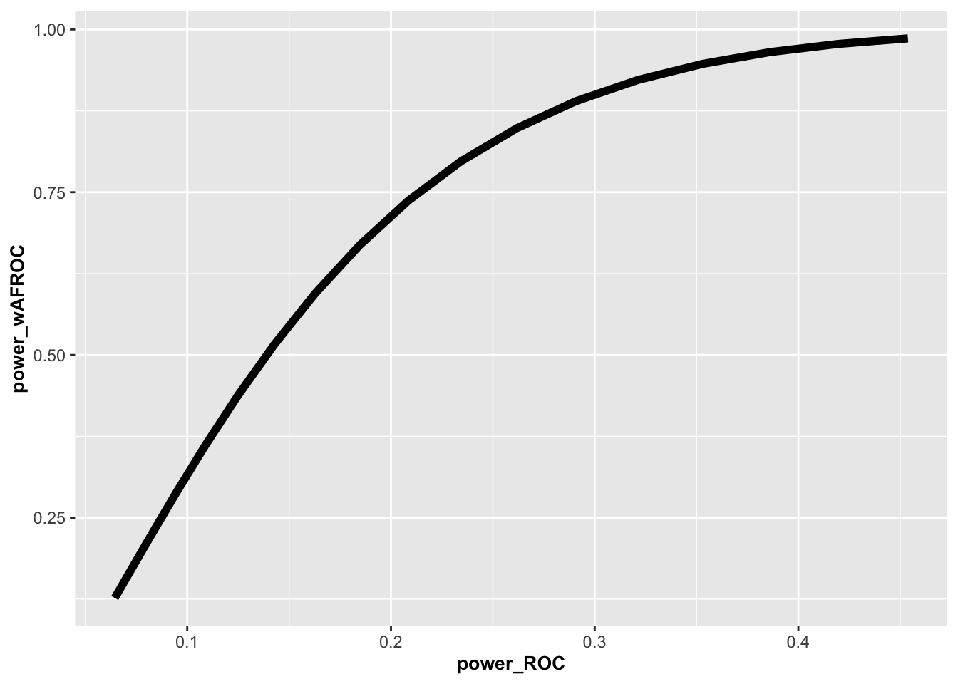
Plot of wAFROC power vs. ROC power. For ROC effect size = 0.035 the wAFROC effect size is 0.0759, the ROC power is 0.234 while the wAFROC power is 0.796.

FIGURE 10.2: Plot of wAFROC power vs. ROC power. For ROC effect size = 0.035 the wAFROC effect size is 0.0759, the ROC power is 0.234 while the wAFROC power is 0.796.

10.4 Part 2

10.4.1 Introduction

This example uses the FED dataset as a pilot FROC study and function SsFrocNhRsmModel() (RSM-based FROC NH model) to construct the NH model (thereby encapsulating some of the code in the first part).

10.4.2 Constructing the NH model

The first two treatments are extracted from dataset04 thereby yielding the NH dataset (line 1). The lesion distribution is specified in line 2. lesDistr can be specified independent of that in the pilot dataset. This allows some control over selection of the diseased cases in the pivotal study. However, in this example it is simply extracted from the pilot dataset. Line 3 constructs the NH model using function SsFrocNhRsmModel to calculate the NH RSM parameters (lines 4 - 6) and the scale factor (line 7).

frocNhData <- DfExtractDataset(dataset04, trts = c(1,2))
lesDistr <- UtilLesDistr(frocNhData) # this can be replaced by the anticipated lesion distribution
ret <- SsFrocNhRsmModel(frocNhData, lesDistr = lesDistr$Freq)
muNH <- ret$mu
lambdaNH <- ret$lambda
nuNH <- ret$nu
scaleFactor <- ret$scaleFactor

The fitting model is defined by muNH = 3.3121491, lambdaNH = 1.714368 and nuNH = 0.7036564 and lesDistr$Freq = 0.69, 0.2, 0.11. The effect size scale factor is scaleFactor = 2.169337. All of these are identical to the Part I values.

10.4.3 Extract the wAFROC variance components

The code applies the significance testing function St() to frocNhData, using FOM = "wAFROC" and extracts the variance components.

varComp_wafroc  <- St(
  frocNhData, 
  FOM = "wAFROC", 
  method = "OR", 
  analysisOption = "RRRC")$ANOVA$VarCom

10.4.4 wAFROC power for specified ROC effect size, number of readers and number of cases

The following example is for ROC effect size = 0.035 (line 1), 5 readers and 100 cases (line 4) in the pivotal study. The function SsPowerGivenJK returns the power for the specified number of readers J (line 9), cases K (line 10) and wAFROC effect size (line 11). Since dataset is set to NULL JStar and KStar (corresponding to the pilot study) and the variance components are supplied as a list variable, lines 12 - 18. If dataset is specified then these are calculated from the pilot study dataset.

effectSizeROC <- 0.035
effectSizewAFROC <- scaleFactor * effectSizeROC

J <- 5;K <- 100 # define pivotal study sample size

ret <- SsPowerGivenJK(
  dataset = NULL, # must set 
  FOM = "wAFROC", 
  J = J, 
  K = K, 
  effectSize = effectSizewAFROC, 
  list(JStar = JStar, 
       KStar = KStar, 
       VarTR = varTR_wafroc,
       Cov1 = Cov1_wafroc,
       Cov2 = Cov2_wafroc,
       Cov3 = Cov3_wafroc,
       Var = Var_wafroc))
power_wafroc <- ret$powerRRRC

## ROC-ES =  0.035 , wAFROC-ES =  0.0759268 , Power-wAFROC =  0.7972539

10.4.5 Number of cases for 80 percent power for a given number of readers

Function SsSampleSizeKGivenJ (number of cases K for desired power for given number of readers J) is shown below. If dataset is set to NULL then JStar and KStar and the variance components must be specified as a list variable, otherwise these are computed from dataset.

SsSampleSizeKGivenJ(
  dataset,
  ...,
  J,
  FOM,
  effectSize = NULL,
  alpha = 0.05,
  desiredPower = 0.8,
)

The following code returns the number of cases needed for 80 percent power for 6 readers (line 3), wAFROC effect size (line 4) = 0.076 and JStar and KStar and wAFROC variance components (lines 5 -11).

ret2 <- SsSampleSizeKGivenJ(
  dataset = NULL, 
  J = 6, 
  effectSize = effectSizewAFROC, 
  list(JStar = JStar, 
       KStar = KStar, 
       VarTR = varTR_wafroc,
       Cov1 = Cov1_wafroc,
       Cov2 = Cov2_wafroc,
       Cov3 = Cov3_wafroc,
       Var = Var_wafroc))

## ROC-ES =  0.035 , wAFROC-ES =  0.0759268 , K80RRRC =  84 , Power-wAFROC =  0.8023879

Here K80RRRC is the number of cases needed for 80 percent power when using RRRC analysis.

REFERENCES

Zanca, Federica, Jurgen Jacobs, Chantal Van Ongeval, Filip Claus, Valerie Celis, Catherine Geniets, Veerle Provost, Herman Pauwels, Guy Marchal, and Hilde Bosmans. 2009. “Evaluation of Clinical Image Processing Algorithms Used in Digital Mammography.” Medical Physics 36 (3): 765–75.