Chapter 12 Empirical AUC

12.1 TBA How much finished

80%

12.2 Introduction

The ROC plot, introduced in Chapter 03, is defined as the plot of sensitivity (y-axis) vs. 1-specificity (x-axis). Equivalently, it is the plot of TPF (y-axis) vs. FPF (x-axis). An equal variance binormal model was introduced which allows an ROC plot to be fitted to a single observed operating point. In Chapter 04, the more commonly used ratings paradigm was introduced.

One of the reasons for fitting observed counts data, such as in Table 4.1 in Chapter 04, to a parametric model, is to derive analytical expressions for the separation parameter \(\mu\) of the model or the area AUC under the curve. Other figures of merit, such as the TPF at a specified FPF, or the partial area to the left of a specified FPF, can also be calculated from this model. Each figure of merit can serve as the basis for comparing two readers to determine which one is better. They have the advantage of being single values, as opposed to a pair of sensitivity-specificity values, thereby making it easier to unambiguously compare performances. Additionally, they often yield physical insight into the task, e.g., the separation parameter is the perceptual signal to noise corresponding to the diagnostic task.

It was shown, TBA Fig. 4.1 (A - B), that the equal variance binormal model did not describe a clinical dataset and that an unequal variance binormal model yielded a better visual fit. This turns out to be an almost universal finding. Before getting into the complexity of the unequal variance binormal model curve fitting, it is appropriate to introduce a simpler empirical approach, which is very popular with some researchers. The New Oxford American Dictionary definition of “empirical” is: “based on, concerned with, or verifiable by observation or experience rather than theory or pure logic”. The method is also termed “non-parametric” as it does not involve any parametric assumptions (specifically normality assumptions). Notation is introduced for labeling individual cases that is used in subsequent chapters. An important theorem relating the empirical area under the ROC to a formal statistic, known as the Wilcoxon, is described. The importance of the theorem derives from its applications to non-parametric analysis of ROC data.

12.3 The empirical ROC plot

The empirical ROC plot is constructed by connecting adjacent observed operating points, including the trivial ones at (0,0) and (1,1), with straight lines. The trapezoidal area under this plot is a non-parametric figure of merit that is threshold independent. Since no parametric assumptions are involved, some prefer it to parametric methods, such as the one to be described in the next chapter. [In the context of AUC, the terms empirical, trapezoidal, or non-parametric all mean the same thing.]

12.3.1 Notation for cases

As in §3.5, cases are indexed by \(k_tt\) where \(t\) indicates the truth-status at the case (i.e., patient) level, with \(t=1\) for non diseased cases and \(t=2\) for diseased cases. Index \(k_1\) ranges from one to \(K_1\) for non-diseased cases and \(k_2\) ranges from one to \(K_2\) for diseased cases, where \(K_1\) and \(K_2\) are the total number of non-diseased and diseased cases, respectively. In Table 5.1, each case is represented as a shaded box, lighter shading for non-diseased cases and darker shading for diseased cases. There are 11 non-diseased cases, labeled N1 – N11, in the upper row of boxes and there are seven diseased cases, labeled D1 – D7, in the lower row of boxes.

TABLE 12.1: On the need for two indices to label cases in an ROC study.

N1	N2	N3	N4	N5	N6	N7	N8	N9	N10	N11
D1	D2	D3	D4	D5	D6	D7

TBA In 12.1 the upper row shows 11 non-diseased cases, labeled N1 – N11, while the lower row shows seven diseased cases, labeled D1 – D7. To address any case one needs two indices: the row number \(t\) and the column number \(k_tt\). Since in general the column number depends on the value of \(t\), one needs two indices to specify the column index. To address a case one needs two indices; the first index is the row number \(t\) and the second index is the column number \(k_tt\). Since the total number of columns depends on the row number, the column index has to be t-dependent, i.e., \(k_tt\), denoting the column index \(k_t\) of a case with truth index \(t\). Alternative notation in more commonly usage uses a single index \(k\) to label the cases. It reserves the first \(K_1\) positions for non-diseased cases and the rest for diseased cases: e.g., \(k = 3\) corresponds to the third non-diseased case, \(k = K_1+5\) corresponds to the fifth diseased case, etc. Because it extends more easily to more complex data structures, e.g., FROC, I prefer the two-index notation.

12.3.2 An empirical operating point

Let \(z_{k_tt}\) represent the z-sample of case \(k_tt\). For a given reporting threshold \(\zeta\), and assuming a positive-directed rating scale (i.e., higher values correspond to greater confidence in presence of disease), empirical false positive fraction \(FPF(\zeta)\) and empirical true positive fraction \(TPF(\zeta)\) are defined by:

\[\begin{equation} \left. \begin{aligned} FPF\left ( \zeta \right ) &= \frac{1}{K_1}\sum_{k_1=1}^{K_1}I\left ( z_{k_11} \geq \zeta \right ) \\ TPF\left ( \zeta \right ) &= \frac{1}{K_2}\sum_{k_2=1}^{K_2}I\left ( z_{k_22} \geq \zeta \right ) \end{aligned} \right \} \tag{12.1} \end{equation}\]

Here \(I(x)\) is the indicator function that equals one if \(x\) is true and is zero otherwise.

In Eqn. (12.1) the indicator functions act as counters, effectively counting instances where the z-sample of a case equals or exceeds \(\zeta\), and division by the appropriate denominator yields the desired left hand sides of these equations. The operating point \(O(\zeta)\) corresponding to threshold \(\zeta\) is defined by:

\[\begin{equation} O\left ( \zeta \right ) = \left ( FPF\left ( \zeta \right ), TPF\left ( \zeta \right ) \right ) \tag{12.2} \end{equation}\]

The essential difference between Eqn. (12.1) and Eqn. (10.18) is that the former is non-parametric while the latter is parametric. In TBA Chapter 03 analytical (or parametric, i.e., model parameter dependent) operating points were obtained. In contrast, here one uses the observed ratings to calculate the empirical operating point.

12.4 Empirical operating points from ratings data

Consider a ratings ROC study with \(R\) bins. Describing an R-rating empirical ROC plot requires \(R-1\) ordered empirical thresholds, see Eqn. (11.5).

The operating point \(O(\zeta_r)\) is given by:

\[\begin{equation} O\left ( \zeta_r \right ) = \left ( FPF\left ( \zeta_r \right ), TPF\left ( \zeta_r \right ) \right ) \tag{12.3} \end{equation}\]

Its coordinates are defined by:

\[\begin{equation} \left. \begin{aligned} FPF_r \equiv FPF\left ( \zeta_r \right )=\frac {1} {K_1} \sum_{k_1=1}^{K_1}I \left ( z_{k_11} \geq \zeta_r\right ) \\ \\ TPF_r \equiv TPF\left ( \zeta_r \right )=\frac {1} {K_2} \sum_{k_2=1}^{K_2} I\left ( z_{k_22} \geq \zeta_r\right ) \end{aligned} \right \} \tag{12.4} \end{equation}\]

For example,

\[\begin{equation} \left. \begin{aligned} FPF_4 \equiv FPF\left ( \zeta_4 \right )=\frac {1} {K_1} \sum_{k_1=1}^{K_1}I \left ( z_{k_11} \geq \zeta_4\right ) \\ \\ TPF_4 \equiv TPF\left ( \zeta_4 \right )=\frac {1} {K_2} \sum_{k_2=1}^{K_2} I\left ( z_{k_22} \geq \zeta_4\right ) \\ O_4 \equiv \left ( FPF_4, TPF_4 \right ) = \left ( 0.017, 0.44 \right )\\ \\ \end{aligned} \right \} \tag{12.5} \end{equation}\]

In Table 11.1 a sample clinical ratings data set was introduced. Shown below is a partial code listing of mainEmpRocPlot.R showing implementation of Eqn. (5.7). Except for the last statement, the plotting part of the code is suppressed.

K1 <- 60
K2 <- 50
FPF <- c(0, cumsum(rev(c(30, 19, 8, 2, 1))) / K1)
TPF <- c(0, cumsum(rev(c(5, 6, 5, 12, 22))) / K2)

ROCOp <- data.frame(FPF = FPF, TPF = TPF)
ROCPlot <- ggplot(
  data = ROCOp, 
  mapping = aes(x = FPF, y = TPF)) + 
  geom_line(size = 1) + 
  geom_point(size = 4) + 
  theme_bw() + 
  theme(panel.grid.major = element_blank(), 
        panel.grid.minor = element_blank(), 
        panel.border = element_rect(color = "black"), 
        axis.text = element_text(size = 15), 
        axis.title = element_text(size = 20)) +
  scale_x_continuous(
    expand = c(0, 0), 
    breaks = c(0.25, 0.5, 0.75, 1)) + 
  scale_y_continuous(
    expand = c(0, 0), breaks = c(0.25, 0.5, 0.75, 1)) +
  coord_cartesian(ylim = c(0,1), x = c(0,1)) + 
  annotation_custom(
    grob = textGrob(bquote(italic("O")),
                    gp = gpar(fontsize = 22)), 
    xmin = -0.03, xmax = -0.03, 
    ymin = -0.03, ymax = -0.03) + 
  annotation_custom(
    grob = textGrob(bquote(italic(O[4])),
                    gp = gpar(fontsize = 22)), 
    xmin = 0.06, xmax = 0.06, 
    ymin = 0.40, ymax = 0.40) +
  annotation_custom(
    grob = textGrob(bquote(italic(O[3])),
                    gp = gpar(fontsize = 22)), 
    xmin = 0.10, xmax = 0.10, 
    ymin = 0.64, ymax = 0.64) +
  annotation_custom(
    grob = textGrob(bquote(italic(O[2])),
                    gp = gpar(fontsize = 22)), 
    xmin = 0.16, xmax = 0.16, 
    ymin = 0.83, ymax = 0.83) +
  annotation_custom(
    grob = textGrob(bquote(italic(O[1])),
                    gp = gpar(fontsize = 22)), 
    xmin = 0.49, xmax = 0.49, 
    ymin = 0.94, ymax = 0.94)  

p <- ggplotGrob(ROCPlot)
p$layout$clip[p$layout$name=="panel"] <- "off"
grid.draw(p)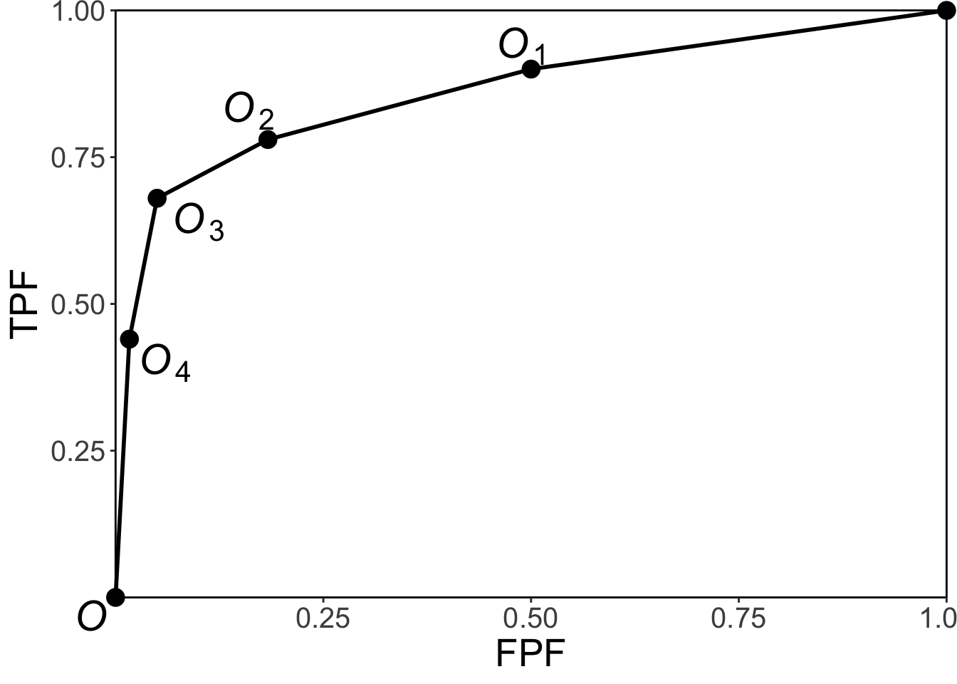

FIGURE 12.1: Empirical ROC plot for the data in Table 4.1. By convention the operating points are numbered starting with the uppermost non-trivial one and working down the plot and the trivial operating points (0,0) and (1,1) are not shown.

The function cumsum() is used to calculate the cumulative sum. The rev() function reverses the order of the array supplied as its argument. The reader should use the debugging techniques (basically copy and paste parts of the code to the Console window and hit enter) to understand how this code implements Eqn. (12.4).

Fig. 12.1 is the empirical ROC plot. It illustrates the convention used to label the operating points introduced in TBA §4.3 is, i.e., \(O_1\) is the uppermost non-trivial point, and the subscripts increment by unity as one moves down the plot. By convention, not shown are the trivial operating points \(O_0 \equiv (FPF_0, TPF_0) = (1,1)\) and \(O_R \equiv (FPF_R, TPF_R) = (0,0)\), where \(R = 5\).

12.5 AUC under the empirical ROC plot

Fig. 12.2 shows the empirical plot for the data in Table 4.1. The area under the curve (AUC) is the shaded area. By dropping imaginary vertical lines from the non-trivial operating points onto the x-axis, the shaded area is seen to be the sum of one triangular shaped area and four trapezoids. One may be tempted to write equations to calculate the total area using elementary algebra, but that would be unproductive. There is a theorem (see below) that the empirical area is exactly equal to a particular statistic known as the Mann-Whitney-Wilcoxon statistic (Wilcoxon 1945; Mann and Whitney 1947), which, in this book, is abbreviated to the Wilcoxon statistic. Calculating this statistic is much simpler than calculating and summing the areas of the triangle and trapezoids, or doing planimetry.

RocDataTable = array(dim = c(2,4))
RocDataTable[1,]  <- c(30,19,8,3)
RocDataTable[2,]  <- c(5,11,12,22)

ret  <- RocOperatingPointsFromRatingsTable( 
  RocDataTable[1,], 
  RocDataTable[2,] )
FPF <- ret$FPF
TPF <- ret$TPF

ROC_Points <- data.frame(FPF = FPF, TPF = TPF)
# add the trivial points
ROC_Points <- rbind(
  c(0, 0), 
  ROC_Points, c(1, 1))

shade <- data.frame(
  FPF = c(ROC_Points$FPF, 1), 
  TPF = c(ROC_Points$TPF, 0))

p <- ggplot(ROC_Points, 
            aes(x = FPF, y = TPF) ) + 
  geom_polygon(data = shade, fill = 'grey') + 
  geom_line(size = 1) + 
  geom_point(size = 4) + 
  theme_bw() + 
  theme(
    panel.grid.major = element_blank(), 
    panel.grid.minor = element_blank()) +
  labs(x = expression(FPF)) + 
  labs(y = expression(TPF)) + 
  scale_x_continuous(expand = c(0, 0)) + 
  scale_y_continuous(expand = c(0, 0)) + 
  coord_cartesian(ylim = c(0,1), x = c(0,1))
print(p)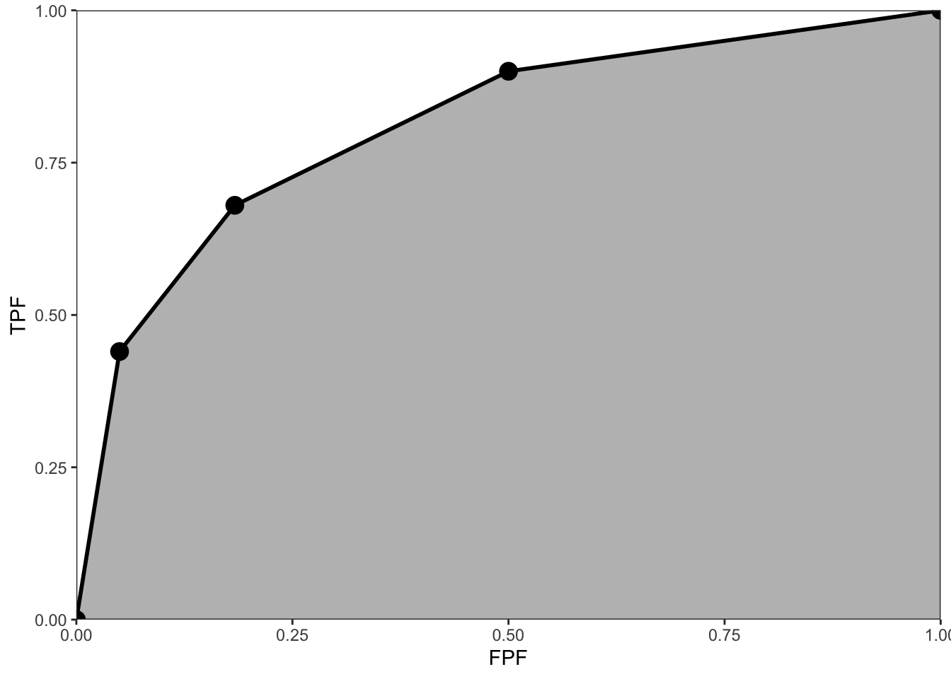

FIGURE 12.2: The empirical ROC plot corresponding to Table 4.1; the shaded area is the area AUC under this plot, a widely used figure of merit in non-parametric ROC analysis.

12.6 The Wilcoxon statistic

A statistic is any value calculated from observed data. The Wilcoxon statistic is defined in terms of the ratings, by:

\[\begin{equation} W=\frac{1}{K_1K_2} \sum_{k_1=1}^{K_1} \sum_{k_2=1}^{K_2} \psi\left ( z_{k_11} , z_{k_22} \right ) \tag{12.6} \end{equation}\]

The function \(\psi\left ( x, y \right )\) is defined by:

\[\begin{equation} \left. \begin{aligned} \psi(x,y)&=1 \qquad & x<y \\ \psi(x,y)&=0.5 & x=y \\ \psi(x,y)&=0 & x>y \end{aligned} \right \} \tag{12.7} \end{equation}\]

The function \(\psi\left ( x, y \right )\) is sometimes called the kernel function. It is unity if the diseased case is rated higher, 0.5 if the two are rated the same and zero otherwise. Each evaluation of the kernel function results from a comparison of a case from the non-diseased set with one from the diseased set. In Eqn. (12.6) the two summations and division by the total number of comparisons yields the observed, i.e., empirical, probability that diseased cases are rated higher than non-diseased ones. Since it is a probability, it can range from zero to one. However, if the observer has any discrimination ability at all, one expects diseased cases to be rated equal or greater than non-diseased ones, so in practice one expects \(0.5 \leq W \leq 1\). The limit 0.5 corresponds to a guessing observer, whose operating point lies on the chance diagonal of the ROC plot.

12.7 Bamber’s Equivalence theorem

The Wilcoxon statistic \(W\) equals the area \(AUC\) under the empirical ROC plot:

\[\begin{equation} W = AUC \tag{12.8} \end{equation}\]

Numerical illustration: While hardly a proof, as an illustration of the theorem it is helpful to calculate the sum on the right hand side of Eqn. (12.6) and compare it to direct integration of the area under the empirical ROC curve (i.e., adding the area of a triangle and several trapezoids). The function is called trapz(x,y), see below. It takes two array arguments, \(x\) and \(y\), where in the current case \(x\) is \(FPF\) and \(y\) is \(TPF\). One has to be careful to include the end-points as otherwise the area will be underestimated. The Wilcoxon \(W\) and the numerical estimate of the empirical area AUC are implemented in the following code.

trapz = function(x, y)
{ ### computes the integral of y with respect to x using trapezoidal integration.
  idx = 2:length(x)
  return (as.double( (x[idx] - x[idx-1]) %*% (y[idx] + y[idx-1])) / 2)
}

Wilcoxon <- function (zk1, zk2)
{
  K1 = length(zk1)
  K2 = length(zk2)
  W <- 0
  for (k1 in 1:K1) {
    W <- W + sum(zk1[k1] < zk2)
    W <- W + 0.5 * sum(zk1[k1] == zk2)
  }
  W <- W/K1/K2
  return (W)
}

RocOperatingPoints <- function( K1, K2 ) {
  
  nOpPts <- length(K1) - 1 # number of op points
  FPF <- array(0,dim = nOpPts)
  TPF <- array(0,dim = nOpPts)
   
  for (r in (nOpPts+1):2) {
    FPF[r-1] <- sum(K1[r:(nOpPts+1)])/sum(K1)
    TPF[r-1] <- sum(K2[r:(nOpPts+1)])/sum(K2)    
  }
  FPF <- rev(FPF)
  TPF <- rev(TPF)
  
  return( list(
    FPF = FPF,
    TPF = TPF
  ) )
}

RocCountsTable = array(dim = c(2,5))
RocCountsTable[1,]  <- c(30,19,8,2,1)
RocCountsTable[2,]  <- c(5,6,5,12,22)

zk1  <- rep(1:length(RocCountsTable[1,]),RocCountsTable[1,])#convert frequency table to array
zk2  <- rep(1:length(RocCountsTable[2,]),RocCountsTable[2,])#do:

w  <- Wilcoxon (zk1, zk2)
cat("The wilcoxon statistic is = ", w, "\n")
#> The wilcoxon statistic is =  0.8606667
ret <- RocOperatingPoints(RocCountsTable[1,], RocCountsTable[2,])
FPF <- ret$FPF;FPF <- c(0,FPF,1)
TPF <- ret$TPF;TPF <- c(0,TPF,1)
AUC <- trapz(FPF,TPF) # trapezoidal integration
cat("direct integration yields AUC = ", AUC, "\n")
#> direct integration yields AUC =  0.8606667

Note the equality of the two estimates.

The following proof is adapted from (Bamber 1975) and while it may appear to be restricted to discrete ratings, the result is in fact quite general, i.e., it is applicable even if the ratings are acquired on a continuous scale. The reason is that in an R-rating ROC study the observed z-samples or ratings take on integer values, 1 through R. If R is large enough, ordering information present in the continuous data is not lost upon binning. In the following it is helpful to keep in mind that one is dealing with discrete distributions of the ratings, described by probability mass functions as opposed to probability density functions, e.g., \(P(Z_2 = \zeta_i)\) is not zero, as would be the case for continuous ratings. The proof is illustrated with Fig. 12.3.

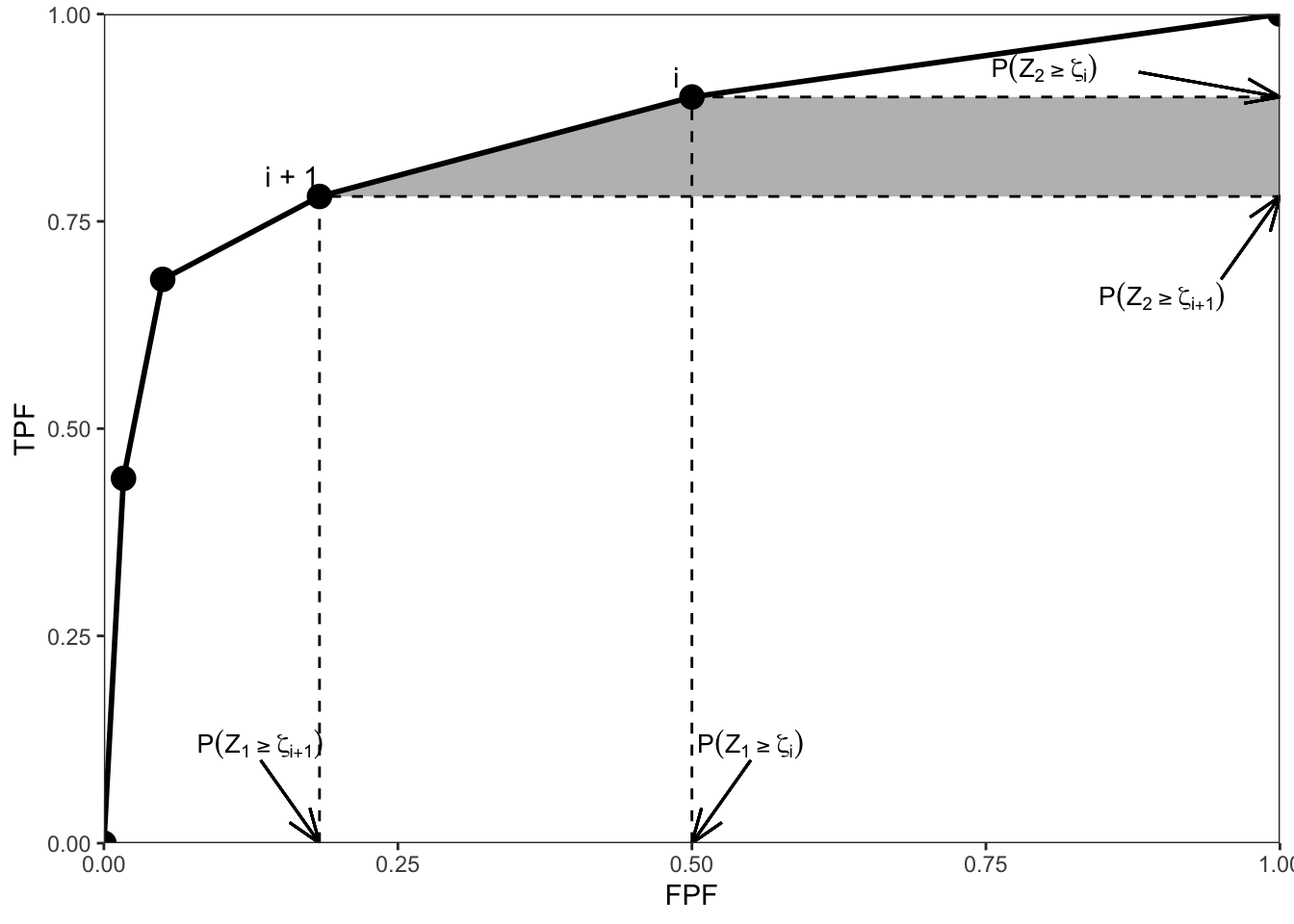
FIGURE 12.3: :Illustration of the derivation of Bamber’s equivalence theorem. Shows an empirical ROC plot for R = 5; the shaded area is due to points labeled i and i + 1.

The abscissa of the operating point \(i\) is \(P(Z_1 \geq \zeta_i)\) and the corresponding ordinate is \(P(Z_2 \geq \zeta_i)\). Here \(Z_1\) is a random sample from a non-diseased case and \(Z_2\) is a random sample from a diseased case. The shaded trapezoid defined by drawing horizontal lines from operating points \(i\) (upper) and \(i+1\) (lower) to the right edge of the ROC plot, Fig. 12.3, has height:

\[\begin{equation} P\left ( Z_2 \geq \zeta_i \right ) - P\left ( Z_2 \geq \zeta_{i+1} \right ) = P\left ( Z_2 = \zeta_i \right ) \tag{12.9} \end{equation}\]

The validity of this equation can perhaps be more easily seen when the first term is written in the form:

\[\begin{equation} P\left ( Z_2 \geq \zeta_i \right ) = P\left ( Z_2 = \zeta_i \right ) + P\left ( Z_2 \geq \zeta_{i+1} \right ) \tag{12.10} \end{equation}\]

The lengths of the top and bottom edges of the trapezoid are, respectively:

\[\begin{equation} 1-P\left ( Z_1 \geq \zeta_i \right )=P\left ( Z_1 < \zeta_i \right ) \tag{12.11} \end{equation}\]

and

\[\begin{equation} 1-P\left ( Z_1 \geq \zeta_{i+1} \right )=P\left ( Z_1 < \zeta_{i+1} \right ) \tag{12.12} \end{equation}\]

The area \(A_i\) of the shaded trapezoid in Fig. 12.3 is (the steps are shown explicitly):

\[\begin{equation} \left. \begin{aligned} A_i &=\frac{1}{2}P\left ( Z_2 = \zeta_i \right )\left [ P\left ( Z_1 < \zeta_i \right ) + P\left ( Z_1 < \zeta_{i+1} \right ) \right ] \\ A_i &=P\left ( Z_2 = \zeta_i \right )\left [ \frac{1}{2}P\left ( Z_1 < \zeta_i \right ) + \frac{1}{2} \left (P\left ( Z_1 = \zeta_i \right ) + P\left ( Z_1 < \zeta_i \right ) \right ) \right ]\\ A_i &=P\left ( Z_2 = \zeta_i \right )\left [ \frac{1}{2} P\left ( Z_1 = \zeta_i \right ) + P\left ( Z_1 < \zeta_i \right ) \right ] \\ \end{aligned} \right \} \tag{12.13} \end{equation}\]

Summing over all values of \(i\), one gets for the total area under the empirical ROC plot:

\[\begin{equation} \left. \begin{aligned} AUC & = \sum_{i=0}^{R-1}A_i\\ & = \frac{1}{2}\sum_{i=0}^{R-1}P\left ( Z_2=\zeta_i \right )P\left ( Z_1=\zeta_i \right )+\sum_{i=0}^{R-1}P\left ( Z_2=\zeta_i \right )P\left ( Z_1<\zeta_i \right ) \end{aligned} \right \} \tag{12.14} \end{equation}\]

It is shown in the Appendix that the term \(A_0\) corresponds to the triangle at the upper right corner of Fig. 12.3, and the term \(A_4\) corresponds to the horizontal trapezoid defined by the lowest non-trivial operating point.

Eqn. (12.14) can be restated as:

\[\begin{equation} AUC=\frac{1}{2}P\left ( Z_1 = Z_2 \right ) + P\left ( Z_1 < Z_2 \right ) \tag{12.15} \end{equation}\]

The Wilcoxon statistic was defined in Eqn. (12.6). It can be seen that the comparisons implied by the summations and the weighting implied by the kernel function are estimating the two probabilities in the expression for in Eqn. (12.15). Therefore, \(AUC = W\).

12.8 Importance of Bamber’s theorem

The equivalence theorem is the starting point for all non-parametric methods of analyzing ROC plots, e.g., (Hanley and Hajian-Tilaki 1997; DeLong, DeLong, and Clarke-Pearson 1988). Prior to Bamber’s work one knew how to plot an empirical operating characteristic and how to calculate the Wilcoxon statistic, but their equality had not been analytically proven. This was Bamber’s essential contribution. In the absence of this theorem, the Wilcoxon statistic would be “just another statistic” in the context of ROC analysis. The theorem is so important that a major paper appeared in Radiology (Hanley and McNeil 1982) devoted to the equivalence. The title of this paper was “The meaning and use of the area under a receiver operating characteristic (ROC) curve”. The equivalence theorem literally gives meaning to the empirical area under the ROC.

12.9 Discussion / Summary

In this chapter, a simple method for estimating the area under the ROC plot has been described. The empirical AUC is a non-parametric measure of performance. Its simplicity and clear physical interpretation as the AUC under the empirical ROC (not fitted, not true) has spurred much theoretical development. These include the De Long et al method for estimating the variance of AUC of a single ROC empirical curve, and comparing pairs of ROC empirical curves5. Bamber’s theorem, namely the equivalence between the empirical AUC and the Wilcoxon statistic has been derived and demonstrated.

Since the empirical AUC always yields a number, the researcher could be unaware about unusual behavior of the empirical ROC curve, so it is always a good idea to plot the data and look for evidence of large extrapolations. An example would be data points clustered at low FPF values, which imply a large AUC contribution, unsupported by intermediate operating points, from the line connecting the uppermost non-trivial operating point to (1,1).

12.10 Appendix 5.A: Details of Wilcoxon theorem

12.10.1 Upper triangle

For \(i = 0\), Eqn. (12.13) implies (since the lowest empirical threshold is unity, the lowest allowed rating, and there are no cases rated less than one):

\[\begin{equation} \left. \begin{aligned} A_0 =& P\left ( Z_2 = 1 \right )\left [ \frac{1}{2} P\left ( Z_1=1 \right ) + P\left ( Z_1<1 \right )\right ] \\ A_0 =& \frac{1}{2} P\left ( Z_1=1 \right ) P\left ( Z_2=1 \right )\\ \end{aligned} \right \} \end{equation}\]

The base of the triangle is:

\[\begin{equation} 1 - P\left ( Z_1 \geq 2 \right )=P\left ( Z_1 < 2 \right )=P\left ( Z_1 = 1 \right ) \end{equation}\]

The height of the triangle is:

\[\begin{equation} 1 - P\left ( Z_2 \geq 2 \right )=P\left ( Z_2 < 2 \right )=P\left ( Z_2 = 1 \right ) \end{equation}\]

Q.E.D.

12.10.2 Lowest trapezoid

For \(i = 4\), Eqn. (12.13) implies:

\[\begin{equation} \left. \begin{aligned} A_4 =& P\left ( Z_2=5 \right )\left [ \frac{1}{2}P\left ( Z_1=5 \right ) + P\left ( Z_1<5 \right )\right ] \\ A_4 =& \frac{1}{2}P\left ( Z_2=5 \right )\left [ P\left ( Z_1=5 \right ) + 2P\left ( Z_1<5 \right )\right ] \\ A_4 =& \frac{1}{2}P\left ( Z_2=5 \right )\left [ P\left ( Z_1=5 \right ) +P\left ( Z_1<5 \right ) + P\left ( Z_1<5 \right )\right ] \\ A_4 =& \frac{1}{2}P\left ( Z_2=5 \right )\left [ 1 + P\left ( Z_1<5 \right )\right ] \\ \end{aligned} \right \} \end{equation}\]

The upper side of the trapezoid is

\[\begin{equation} 1-P\left ( Z_1 \geq 5 \right )= P\left ( Z_1 < 5 \right ) \end{equation}\]

The lower side is unity. The average of the two sides is:

\[\begin{equation} \frac{1 + P\left ( Z_1 < 5 \right )}{2} \end{equation}\]

The height is:

\[\begin{equation} P\left ( Z_2 \geq 5 \right ) = P\left ( Z_2 = 5 \right ) \end{equation}\]

Multiplication of the last two expressions yields \(A_4\).

12.11 References

References

Bamber, Donald. 1975. “The Area Above the Ordinal Dominance Graph and the Area Below the Receiver Operating Characteristic Graph.” Journal Article. Journal of Mathematical Psychology 12 (4): 387–415. https://doi.org/10.1016/0022-2496(75)90001-2.

DeLong, E. R., D. M. DeLong, and D. L. Clarke-Pearson. 1988. “Comparing the Areas Under Two or More Correlated Receiver Operating Characteristic Curves: A Nonparametric Approach.” Journal Article. Biometrics 44: 837–45. https://doi.org/10.2307/2531595.

Hanley, J. A., and B. J. McNeil. 1982. “The Meaning and Use of the Area Under a Receiver Operating Characteristic (ROC) Curve.” Journal Article. Radiology 143 (1): 29–36. http://radiology.rsnajnls.org/cgi/content/abstract/143/1/29.

Hanley, James A., and Karim O. Hajian-Tilaki. 1997. “Sampling Variability of Nonparametric Estimates of the Areas Under Receiver Operating Characteristic Curves: An Update.” Journal Article. Academic Radiology 4 (1): 49–58. https://doi.org/10.1016/s1076-6332(97)80161-4.

Mann, H. B., and D. R. Whitney. 1947. “On a Test of Whether One of Two Random Variables Is Stochastically Larger Than the Other.” Journal Article. Annals of Mathematical Statistics 18: 50−60.

Wilcoxon, F. 1945. “Individual Comparison by Ranking Methods.” Journal Article. Biometrics 1: 80–83.