Chapter 24 The FROC paradigm

24.1 TBA How much finished

70%

24.2 Introduction

Until now the focus has been on the receiver operating characteristic (ROC) paradigm. For diagnostic tasks such as detecting diffuse interstitial lung disease⁹, or diseases similar to it, where disease location is implicit – by definition diffuse interstitial lung disease is spread through, and confined to, lung tissues – this is an appropriate paradigm in the sense that essential information is not being lost by limiting the radiologist’s response in the study to a single rating categorizing the likelihood of presence of interstitial disease.

In clinical practice it is not only important to identify if the patient is diseased, but also to offer further guidance to subsequent care-givers regarding other characteristics (such as type, location, size, extent) of the disease. In most clinical tasks, if the radiologist believes the patient may be diseased, there is a location (or more than one location) associated with the manifestation of the suspected disease. Physicians have a term for this: focal disease: disease located at a specific region of the image.

For focal disease, the ROC paradigm restricts the collected information to a single rating representing the confidence level that there is disease somewhere in the patient’s imaged anatomy. The emphasis on “somewhere” is because it begs the question: if the radiologist believes the disease is somewhere, why not have them to point to it? In fact they do “point to it” in the sense that they record the location(s) of suspect regions in their clinical report, but the ROC paradigm cannot use this information. Clinicians have long recognized problems with ignoring location (Black and Dwyer 1990; Black 2000). Neglect of location information leads to loss of statistical power: the basic reason for this is that there is additional noise in the measurement due to crediting the reader for correctly detecting the diseased patient but getting the wrong lesion location - i.e., being right for the wrong reason. One way of compensating for reduced statistical power is to increase the sample size, which increases the cost of the study and is also unethical because, by not using the optimal paradigm and analysis, one is subjecting more patients to imaging procedures (Halpern, Karlawish, and Berlin 2002).

Here is an outline of this chapter. Four observer performance paradigms are compared, using a visual schematic, as to the kinds of information collected and ignored. An essential characteristic of the FROC paradigm, namely visual search, is introduced. The FROC paradigm and its historical context is described. A pioneering FROC study using phantom images is described. Key differences between FROC ratings and ROC data are noted. The FROC plot is introduced. The dependence of population and empirical FROC plots on a variable identified as perceptual signal-to-noise-ratio (pSNR) is shown. The expected dependence of the FROC curve on pSNR is illustrated with a “solar” analogy – understanding this is key to obtaining a good intuitive feel for this paradigm. The finite extent of the FROC curve, characterized by an end-point, is noted.

The starting point is a comparison of four observer performance paradigms.

24.3 Location specific paradigms

Location-specific paradigms take into account, to varying degrees, information regarding the locations of perceived lesions, so they are sometimes referred to as lesion-specific (or lesion-level) paradigms (Alberdi et al. 2008). Usage of this term is discouraged. In this book the term “lesion” is reserved for true malignant lesions (as distinct from “perceived lesions” or “suspicious regions” that may not be true lesions).

All observer performance methods involve detecting the presence of true lesions; so ROC methodology is, in this sense, also lesion-specific. On the other hand location is a characteristic of true and perceived focal lesions, and methods that account for location are better termed location-specific than lesion-specific. There are three location-specific paradigms:

the free-response ROC (FROC) (Philip C Bunch et al. 1977; Chakraborty 1989);
the location ROC (LROC) (Starr, Metz, and Lusted 1977; Richard G. Swensson 1996);
the region of interest (ROI) (Obuchowski, Lieber, and Powell 2000).

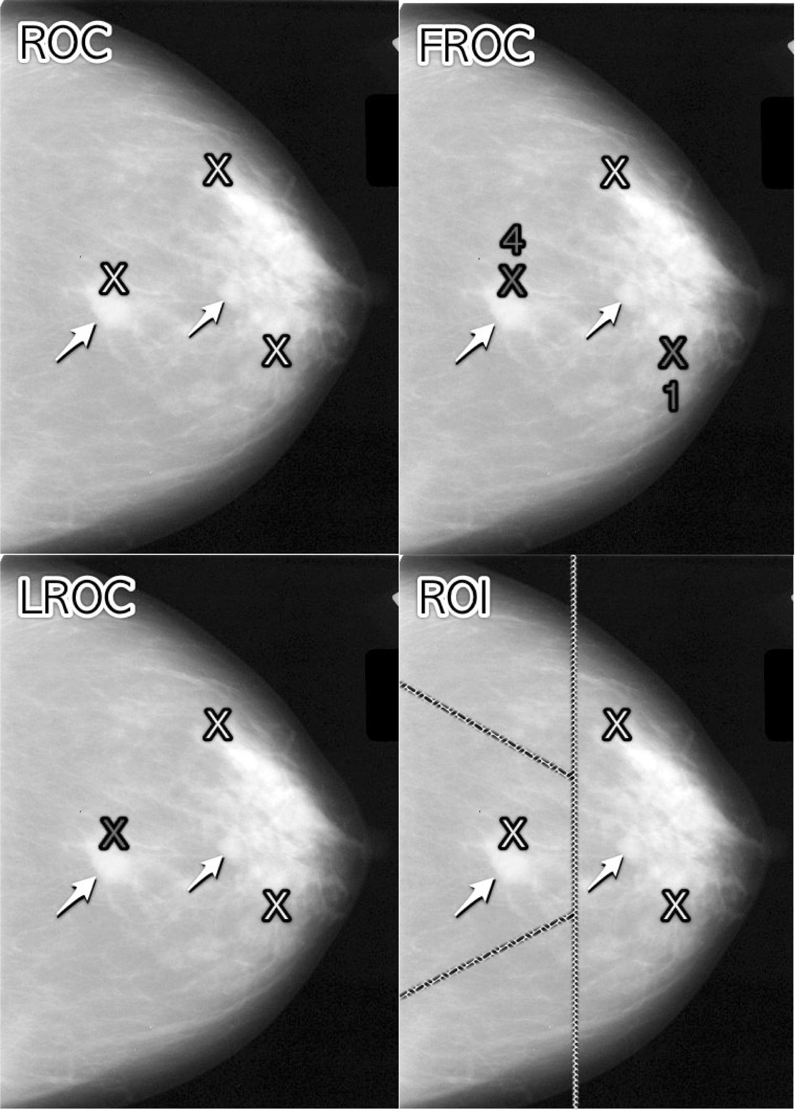
FIGURE 24.1: Upper Left: ROC, Upper Right: FROC, Lower Left: LROC, Lower Right: ROI

Fig. 24.1 shows a schematic mammogram interpreted according to current observer performance paradigms. The arrows point to two real lesions and the three light crosses indicate suspicious regions. Evidently the radiologist saw one of the lesions, missed the other lesion and mistook two normal structures for lesions.

ROC (top-left): the radiologist assigns a single rating that the image contains at least one lesion, somewhere.
FROC (top-right): the dark crosses indicate suspicious regions that are marked and the accompanying numerals are the FROC ratings.
LROC (bottom-left): the radiologist provides a single rating that the the image contains at least one lesion and marks the most suspicious region.
ROI (bottom-right): the image is divided – by the researcher – into a number of regions-of-interest (ROIs) and the radiologist rates each ROI for presence of at least one lesion somewhere within the ROI.

The numbers and locations of suspicious regions depend on the case and the radiologists’ expertise level. Some images can be correctly perceived as obviously non-diseased so that expert radiologists perceive nothing suspicious in them, or they can be correctly perceived as obviously diseased and the suspicious regions are so conspicuous that they are correctly localized by the expert radiologist. There is the gray area – especially when lesions are of low conspicuity – where two radiologists may perceive different suspicious regions, not all lesions present are perceived, and/or false regions are perceived as lesions.

In Fig. 24.1, evidently the radiologist found one of the lesions (the lightly shaded cross near the left most arrow), missed the other one (pointed to by the second arrow) and mistook two normal structures for lesions (the two lightly shaded crosses that are relatively far from any true lesion). The term lesion always refers to a true or real lesion. The prefix “true” or “real” is implicit. The term suspicious region is reserved for any region that, as far as the observer is concerned, has “lesion-like” characteristics. A lesion is a real while a suspicious region is perceived.

In the ROC paradigm, Fig. 24.1 (top-left), the radiologist assigns a single rating indicating the confidence level that there is at least one lesion somewhere in the image. Assuming a 1 – 5 positive directed integer rating scale, if the left-most lightly shaded cross is a highly suspicious region then the ROC rating might be 5 (highest confidence for presence of disease).
In the free-response (FROC) paradigm, Fig. 24.1 (top-right), the dark shaded crosses indicate suspicious regions that were marked (or reported in the clinical report), and the adjacent numbers are the corresponding ratings, which now apply to specific regions in the image, unlike ROC where the rating applies to the whole image. Assuming the allowed FROC ratings are 1 through 4, two marks are shown, one rated FROC-4, which is close to a true lesion, and the other rated FROC-1, which is not close to any true lesion. The third suspicious region, indicated by the lightly shaded cross, was not marked, implying its confidence level did not exceed the lowest reporting threshold. The marked region rated FROC-4 (highest FROC confidence) is likely what caused the radiologist to assign the ROC-5 rating to this image in the top-left ROC paradigm figure.
In the LROC paradigm, Fig. 24.1 (bottom-left), the radiologist provides a rating summarizing confidence that there is at least one lesion somewhere in the image (as in the ROC paradigm) and marks the most suspicious region in the image. In this example the rating might be LROC-5, the five rating being the same as in the ROC paradigm, and the mark may be the suspicious region rated FROC-4 in the FROC paradigm, and, since it is close to a true lesion, in LROC terminology it would be recorded as a correct localization. If the mark were not near a lesion it would be recorded as an incorrect localization. Only one mark is allowed in this paradigm, and in fact one mark is required on every image, even if the observer does not find any suspicious regions to report. The late Prof. Swensson has been the prime contributor to this paradigm.
In the region of interest (ROI) paradigm, the researcher segments the image into a number of regions-of-interest (ROIs) and the radiologist rates each ROI for presence of at least one suspicious region somewhere within the ROI. The rating is similar to the ROC rating, except it applies to the segmented ROI, not the whole image. Assuming a 1 – 5 positive directed integer rating scale in Fig. 24.1 (bottom-right) there are four ROIs. The ROI at ~9 o’clock might be rated ROI-5 as it contains the most suspicious light cross, the one at ~11 o’clock might be rated ROI-1 as it does not contain any light crosses, the one at ~3 o’clock might be rated LROC-2 or 3 (the unmarked light cross would tend to increase the confidence level) and the one at ~7 o’clock might be rated ROI-1. In the example shown in Fig. 24.1 (bottom-right), each case yields 4 ratings. Prof. Obuchowski has been the principal contributor to this paradigm.¹⁰

The rest of this book part focuses on the FROC paradigm.

24.4 Visual search

The FROC paradigm in medical imaging is equivalent to a visual search task. Any search task has two components: (i) finding something and (ii) acting on it. An example of a search task is looking for lost car-keys or a milk carton in the refrigerator. Success in a search task is finding the searched for object. Acting on it could be driving to work or drinking milk from the carton. There is search-expertise associated with any search task. Husbands are notoriously bad at finding the milk carton in the refrigerator (analogy due to Dr. Elizabeth Krupinski at an SPIE course taught jointly with me). Like anything else, search expertise is honed by experience, i.e., lots of practice.

Likewise, a medical imaging search task has two components (i) finding suspicious regions and (ii) acting on each finding (“finding”, used as a noun, is the actual term used by clinicians in their reports), i.e., determining the relevance of each finding to the health of the patient, and whether to report it. A general feature of a medical imaging search task is that the radiologist does not know a-priori if the patient is diseased and, if diseased, how many lesions are present. In the breast-screening context, it is known a-priori that about 5 out of 1000 cases have cancers, so 99.5% of the time odds are that the case has no malignant lesions.¹¹ The radiologist searches each image for lesions. If a suspicious region is found, and provided it is sufficiently suspicious, the relevant location is marked and rated for confidence in being a lesion. The process is repeated for each suspicious region found in the case. A screening mammography report consists of a listing of search related findings. To summarize: Free-response data consists of a variable number of mark-rating pairs per case.

24.4.1 Proximity criterion and scoring the data

In the first two clinical applications of the FROC paradigm (Chakraborty et al. 1986; Niklason et al. 1986) the marks and ratings were indicated by a grease pencil on an acrylic overlay aligned, in a reproducible way, to the CRT displayed chest image. Credit for a correct detection and localization, termed a lesion-localization or LL-event,¹² was given only if a mark was sufficiently close (as per proximity criterion, see below) to an actual diseased region; otherwise, the observer’s mark-rating pair was scored as a non-lesion localization or NL-event.

The use of ROC terminology, such as true positives or false positives to describe FROC data is not conducive to clarity, and is strongly discouraged.
The classification of each mark as either a LL or a NL is referred to as scoring the marks.

Definition:

NL = non-lesion localization, i.e., a mark that is not close to any lesion
LL = lesion localization, i.e., a mark that is close to a lesion

What is meant by sufficiently close? One adopts an acceptance radius (for spherical lesions) or proximity criterion (the more general case). What constitutes “close enough” is a clinical decision the answer to which depends on the application. It is not necessary for two radiologists to point to the same pixel in order for them to agree that they are seeing the same suspicious region. Likewise, two physicians – e.g., the radiologist finding the lesion on an x-ray and the surgeon responsible for resecting it – do not have to agree on the exact center of a lesion in order to appropriately assess and treat it. More often than not, “clinical common sense” can be used to determine if a mark actually localized the real lesion. When in doubt, the researcher should ask an independent radiologist (i.e., not one used in the observer study) how to score ambiguous marks. A rigid definition of the proximity criterion should not be used.

For roughly spherical nodules a simple rule can be used. If a circular lesion is 10 mm in diameter, one can use the “touching-coins” analogy to determine the criterion for a mark to be classified as lesion localization. Each coin is 10 mm in diameter, so if they touch, their centers are separated by 10 mm, and the rule is to classify any mark within 10 mm of an actual lesion center as a LL mark, and if the separation is greater, the mark is classified as a NL mark. A recent paper (Dobbins III et al. 2016) using FROC analysis gives more details on appropriate proximity criteria in the clinical context.¹³

24.4.2 Multiple marks in the same vicinity

Multiple marks near the same vicinity are rarely encountered with radiologists, especially if the perceived lesion is mass-like.¹⁴ However, algorithmic readers, such as CAD, tend to find multiple regions in the same area. Algorithm designers generally incorporate a clustering step to reduce overlapping regions to a single region and assign the highest rating to it (i.e., the rating of the highest rated mark, not the rating of the closest mark.¹⁵

24.4.3 Historical context

The term “free-response” was coined by (Egan, Greenburg, and Schulman 1961) to describe a task involving the detection of brief audio tone(s) against a background of white-noise (white-noise is what one hears if an FM tuner is set to an unused frequency). The tone(s) could occur at any instant within an active listening interval, defined by an indicator light bulb that is turned on. The listener’s task was to respond by pressing a button at the specific instant(s) when a tone(s) was perceived (heard). The listener was uncertain how many true tones could occur in an active listening interval and when they might occur. Therefore, the number of responses (button presses) per active interval was a priori unpredictable: it could be zero, one or more. The Egan et al study did not require the listener to rate each button press, but apart from this difference and with a two-dimensional image replacing the listening interval, the acoustic signal detection study is similar to a common task in medical imaging, namely, prior to interpreting a screening case for possible breast cancer, the radiologist does not know how many diseased regions are actually present and, if present, where they are located. Consequently the case (all 4 views and possibly prior images) is searched for regions that appear to be suspicious for cancer. If one or more suspicious regions are found, and the level of suspicion of at least one of them exceeds the radiologists’ minimum reporting threshold, the radiologist reports the region(s). At my former institution (University of Pittsburgh, Department of Radiology) the radiologists digitally outline and annotate (describe) suspicious region(s) that are found. As one would expect from the low prevalence of breast cancer, in the screening context about 5 per 1000 cases in the US, and assuming expert-level radiologist interpretations, about 90% of breast cases do not generate any marks, implying case-level specificity of 90%. About 10% of cases generate one or more marks and are recalled for further comprehensive imaging (termed diagnostic workup). Of marked cases about 90% generate one mark, about 10% generate 2 marks, and a rare case generates 3 or more marks. Conceptually, a mammography report consists of the locations of regions that exceed the threshold and the corresponding levels of suspicion, reported as a Breast Imaging Reporting and Data System (BIRADS) rating (the BIRADS rating is actually assigned after the diagnostic workup following a 0-screening rating; the screening rating itself is binary: 0 for recall or 1 for normal).

Described next is the first medical imaging application of this paradigm.

24.5 A pioneering FROC study in medical imaging

This section details an FROC paradigm phantom study with x-ray images conducted in 1978 that is often overlooked. With the obvious substitution of clinical images for the phantom images, this study is a template for how an FROC experiment should be conducted. A detailed description of it is provided to set up the paradigm, the terminology used to describe it, and to introduce the FROC plot.

24.5.1 Image preparation

Bunch et al. conducted the first radiological free-response paradigm study using simulated lesions. They drilled 10-20 small holes (the simulated lesions) at random locations in ten 5 cm x 5 cm x 1.6 mm Teflon sheets. A Lucite plastic block 5 cm thick was placed on top of each Teflon sheet to decrease contrast and increase scatter, thereby appropriately reducing visibility of the holes (otherwise the hole detection task would be too easy; as in ROC it is important that the task not be too easy or too difficult). Imaging conditions (kVp, mAs) were chosen such that, in preliminary studies, approximately 50% of the simulated lesions were correctly localized at the observer’s lowest confidence level. To minimize memory effects, the sheets were rotated, flipped or replaced between exposures. Six radiographs of 4 adjacent Teflon sheets, arranged in a 10 cm x 10 cm square, were obtained. Of these six radiographs one was used for training purposes, and the remaining five for actual data collection. Contact radiographs (i.e., with high visibility of the simulated lesions) of the sheets were obtained to establish the true lesion locations. Observers were told that each sheet contained from 0 to 30 simulated lesions. A mark had to be within about 1 mm to count as a correct localization; a rigid definition was deemed unnecessary. Once images had been prepared, observers interpreted them.

24.5.2 Image Interpretation and the 1-rating

Observers viewed each film and marked and rated any visible holes with a felt-tip pen on a transparent overlay taped to the film at one edge (this allowed the observer to view the film directly without the distracting effect of previously made marks – in digital interfaces it is important to implement a show/hide feature in the user interface). The record of mark-rating pairs generated by the observer constitutes free-response data.

The observers used a 4-point ordered rating scale with 4 representing “most likely a simulated lesion” to 1 representing “least likely a simulated lesion”. Note the meaning of the 1 rating: least likely a simulated lesion. There is confusion with some using the FROC-1 rating to mean “definitely not a lesion”. If that were the observer’s understanding, then logically the observer would “fill up” the entire image, especially parts outside the patient anatomy, with 1’s, as each of these regions is “definitely not a lesion”. Since the observer did not behave in this unreasonable way, the meaning of the FROC-1 rating, as they interpreted it, or were told, must have been “I have nothing further to report on this image”.

When correctly used, the 1-rating means there is some finite, perhaps small, probability that the marked region is a lesion. In this sense the free-response rating scale is asymmetric. Compare the 5 rating ROC scale, where ROC-1 = “patient is definitely not diseased” and ROC-5 = “patient definitely diseased”. This is a symmetric confidence level scale. In contrast the free-response confidence level scale labels different confidence levels of positivity in presence of disease. Table 24.1 compares the ROC 5-rating study to a FROC 4-rating study.

Table 24.1: comparison of ROC and FROC rating scales: note that the FROC rating is one less than the corresponding ROC rating and that there is no rating corresponding to ROC-1 The observer’s way of indicating definitely non-diseased images is by simply not marking them. (NA = not available.)

TABLE 24.1: Comparison of ROC and FROC rating scales: note that the FROC rating is one less than the corresponding ROC rating and that there is no rating corresponding to ROC-1.
ROC Rating	Observer’s Description	FROC Rating	Observer’s Description
1	Definitely not diseased	NA	Image is not marked
2	Probably not diseased	1	Just possible it is a lesion
3	Possibly diseased	2	Possibly a lesion
4	Probably diseased	3	Probably a lesion
5	Definitely diseased	4	Definitely a lesion

The FROC rating is one less than the corresponding ROC rating because the ROC-1 rating is not used by the observer; the observer indicates such images by the simple expedient of not marking them.

24.5.3 Scoring the data

Scoring the data was defined 24.4.1 as the process of classifying each mark-rating pair as NL or LL according to the chosen proximity criterion. In the Bunch et al study, after each case was read the person running the study (i.e., Dr. Phil Bunch) compared the marks on the overlay to the true lesion locations on the contact radiographs and scored the marks as lesion localizations (LLs: lesions correctly localized to within about 1 mm radius) or non-lesion localizations (NLs: all other marks).¹⁶

24.6 The free-response receiver operating characteristic (FROC) plot

The free-response receiver operating characteristic (FROC) plot was introduced, also in an auditory detection task, by Miller (Miller 1969) as a way of visualizing performance in the free-response auditory tone detection task. In the medical imaging context, assume the mark rating pairs have been classified as NLs (non-lesion localizations) or LLs (lesion localizations).

Non-lesion localization fraction (NLF) is defined as the total number of NLs rated at or above a threshold rating divided by the total number of cases.
Lesion localization fraction (LLF) is defined as the total number of LLs rated at or above the same threshold rating divided by the total number of lesions in the case set.
The FROC plot is defined as that of LLF (ordinate) vs. NLF as the threshold is varied. Unlike the ROC plot which is completely contained in the unit square, the FROC plot is not.
The upper-right most operating point is termed the observed end-point and its coordinated are denoted $(\text{NLF}_{\text{max}}, \text{LLF}_{\text{max}})$.

While the ordinate LLF is a proper fraction, e.g., 30/40 assuming 30 LLs and 40 true lesions, the abscissa is an improper fraction that can exceed unity, like 35/21 assuming 35 NLs on 21 cases). The NLF notation is not ideal: as will become evident in the next chapter, it is used for notational symmetry and compactness.

Following Miller’s suggestion, (Philip C Bunch et al. 1977, @bunch1977freeSPIE) plotted lesion localization fraction (LLF) along the ordinate vs. non-lesion localization fraction (NLF) along the abscissa. Corresponding to the different threshold ratings, pairs of (NLF, LLF) values, or operating points on the FROC, were plotted. For example, in a positive directed four-rating FROC study, such as employed by Bunch et al, 4 FROC operating points resulted: that corresponding to marks rated 4s; that corresponding to marks rated 4s or 3s; the 4s, 3s, or 2s; and finally the 4s, 3s, 2s, or 1s. An R-rating (integer R > 0) FROC study yields at most R operating points. So Bunch et al were able to plot only 4 operating points per reader, Fig. 6 ibid. Lacking a method of fitting a continuous FROC curve to the operating points, they did the best they could, and manually “French-curved” fitted curves. In 1986, I followed the same practice in my first paper on this topic (Chakraborty et al. 1986). In 1989 I described (Chakraborty 1989) a method for fitting such operating points, and developed software called FROCFIT, but the fitting method is obsolete, as the underlying statistical model has been superseded, and moreover, it is now known that the FROC plot is a poor visual descriptor of performance.

If continuous ratings are used, the procedure is to start with a very high threshold so that none of the ratings exceed the threshold, and one gradually lowers the threshold. Every time the threshold crosses the rating of a mark, or possibly multiple marks, the total count of LLs and NLs exceeding the threshold is divided by the appropriate denominators yielding the ‘’raw’’ FROC plot. For example, when an LL rating just exceeds the threshold, the operating point jumps up by 1/(total number of lesions), and if two LLs simultaneously just exceed the threshold, the operating point jumps up by 2/(total number of lesions). If an NL rating just exceeds the threshold, the operating point jumps to the right by 1/(total number of cases). If an LL rating and a NL rating simultaneously just exceed the threshold, the operating point moves diagonally, up by 1/(total number of lesions) and to the right by 1/(total number of cases). The reader should get the general idea by now and recognize that the cumulating procedure is very similar to the manner in which ROC operating points were calculated, the only differences being in the quantities being cumulated and the relevant denominators.

Having seen how a binned data FROC study is conducted and scored, and the results “French-curved” as an FROC plot, typical simulated plots, generated under controlled conditions, are shown next, both for continuous ratings data and for binned rating data. Such demonstrations, that illustrate basic principles and trends, are impossible using real datasets. The reader should take my word for it (for now) that the radiological search model (RSM) simulator used is the simplest one possible that incorporates key elements of the search process. Details of the simulator are given in TBA Chapter 16, but for now the following summary should suffice.

24.7 Preview of the RSM data simulator

The RSM simulator is characterized by three parameters $\mu$, $\lambda$ and $\nu$. The parameter $\nu$ characterizes the ability of the observer to find lesions (larger values preferred), the $\lambda$ parameter characterizes the ability of the observer to avoid finding non-lesions (smaller values preferred) and parameter $\mu$ characterizes the ability of the observer to correctly classify a found suspicious region as a true lesion or a non-lesion (larger values preferred). The reader may think of $\mu$ as a perceptual signal-to-noise ratio (pSNR) or conspicuity of the lesion (similar to the separation parameter of the binormal model) that separates two normal distributions describing the z-sampling of ratings of NLs and LLs. Finally, there is a threshold parameter $\zeta_1$ that determines if a found suspicious region is actually marked. If $\zeta_1$ is negative infinity, then all found suspicious regions are marked and conversely, as $\zeta_1$ increases, only those suspicious regions whose z-samples exceed $\zeta_1$ are marked.

24.8 Population and binned FROC plots

Fig. 24.3 (A - C) shows simulated population FROC plots when the ratings are not binned, i.e., raw FROC plots, where the ratings were generated by the RJafroc function SimulateFrocDataset(). The help page for this function is shown below.

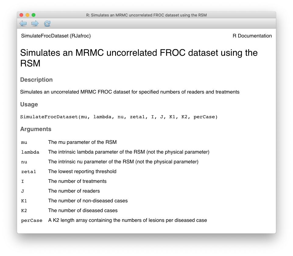
FIGURE 24.2: Help page for RJafroc function SimulateFrocDataset

For now ignore the distinction between intrinsic and physical parameters. As evident from the following code, one supplies the function with the parameters of the RSM: $\mu, \lambda, \nu$, the threshold parameter $\zeta_1 = -\infty$, the number of treatments $I = 1$, the number of readers $J = 1$, the number of non-diseased cases $K_1$, the number of diseased cases $K_2$, and the number of lesions per each diseased case Lk2. In this example the maximum number of lesions per case Lmax has been specified to be two.

Single modality single reader FROC data from 10,000 non-diseased and 10,000 diseased were generated by SimulateFrocDataset()(the code takes a while to finish). The very large number of cases minimizes sampling variability, thereby approximating “population” curves. Additionally, the reporting threshold was set to negative infinity to ensure that all suspicious regions were marked. Plots (A) – (C) correspond to $\mu$ equal to 0.5, 1 and 2, respectively, were generated by PlotEmpiricalOperatingCharacteristics().

seed <- 1
set.seed(seed)
mu_arr <- c(0.5, 1, 2) # the three selected values of mu
lambda <- 1
nu <- 1 
zeta1 <- -Inf
K1 <- 1000
K2 <- 1000
Lmax <- 2 # maximum number of lesions per case
Lk2 <- floor(runif(K2, 1, Lmax + 1)) # no. les. per dis. case

for (i in 1:3) {
  mu <- mu_arr[i]
  frocDataRaw <- SimulateFrocDataset(
    mu = mu, 
    lambda = lambda, 
    nu = nu, 
    zeta1 = zeta1,
    I = 1, 
    J = 1, 
    K1 = K1, 
    K2 = K2, 
    perCase = Lk2 
  )
  
  frocRaw <- PlotEmpiricalOperatingCharacteristics(
    dataset = frocDataRaw, 
    trts= 1, 
    rdrs = 1, 
    opChType = "FROC", 
    legend.position = "NULL")
  
  if (i == 1) figA <- frocRaw$Plot + ggtitle("A")
  if (i == 2) figB <- frocRaw$Plot + ggtitle("B")
  if (i == 3) figC <- frocRaw$Plot + ggtitle("C")
}

Plots (D) – (F) correspond to 5-ratings binned data for 50 non-diseased and 70 diseased cases, and the same values of the RSM parameters as in the preceding example. The binning was performed using function DfBinDataset(). [Binning 20,000 cases requires much more time and is not useful.]

K1 <- 50
K2 <- 70
Lk2 <- floor(runif(K2, 1, Lmax + 1))
for (i in 1:3) {
  mu <- mu_arr[i]
  frocDataRaw1 <- SimulateFrocDataset(
    mu = mu, 
    lambda = lambda, 
    nu = nu, 
    zeta1 = zeta1,
    I = 1, 
    J = 1, 
    K1 = K1, 
    K2 = K2, 
    perCase = Lk2 
  )
  frocDataBin <- DfBinDataset(frocDataRaw1, desiredNumBins = 5, opChType = "FROC")
  
  frocBin <- PlotEmpiricalOperatingCharacteristics(
    dataset = frocDataBin, 
    trts= 1, 
    rdrs = 1, 
    opChType = "FROC", 
    legend.position = "NULL")
  
  if (i == 1) figD <- frocBin$Plot + ggtitle("D")
  if (i == 2) figE <- frocBin$Plot + ggtitle("E")
  if (i == 3) figF <- frocBin$Plot + ggtitle("F")
}

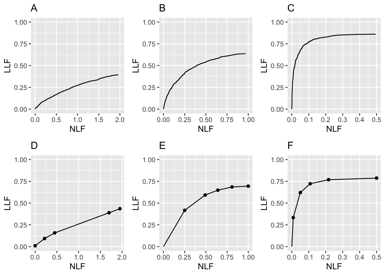
FIGURE 24.3: FROC plots: A, B, C correspond to raw population plots and D, E, F to binned plots with fewer cases.

Fig. 24.3: Plots (A) – (C): Population FROC plots for $\mu$ = 0.5, 1, 2; the other parameters are $\lambda$ = 1, $\nu$ = 1, $\zeta_1 = -\infty$ and $L_{\text{max}} = 2$ is the maximum number of lesions per case in the dataset. Plots (D) – (F) correspond to 50 non-diseased and 70 diseased cases, where the data was binned into 5 bins, and other parameters are unchanged. As $\mu$ increases, the uppermost point moves upwards and to the left (the latter trend is somewhat hidden by the changing scale factor of the x-axis).

Points to note:

Plots (A) – (C) show quasi-continuous plots, while (D) – (F) show operating points, five per plot, connected by straight line segments, so they are termed empirical FROC curves, analogous to the empirical ROC curves encountered in previous chapters. At a “microscopic level” plots (A) – (C) are also discrete, but one would need to “zoom in” to see the discrete behavior (upward and rightward jumps) as each rating crosses a sliding threshold.
The empirical plots in the bottom row (D - F) are subject to sampling variability and will not, in general, match the population plots. The reader may wish to experiment with different values of the seed variable in the code.
In general FROC plots do not extend indefinitely to the right.¹⁷

Like an ROC plot, the population FROC curve rises monotonically from the origin, initially with infinite slope (this may not be visually evident for Fig. 24.3 (A), but it is true, see next code segment). If all suspicious regions are marked, i.e., $\zeta_1 = -\infty$, the plot reaches its upper-right most limit, termed the end-point, with zero slope (again, this may not be visually evident for (A), but it is true). In general these characteristics, i.e., initial infinite slope and zero final slope, are not true for the empirical plots Fig. 24.3 (D – F).

y <- frocRaw$Points$genOrdinate
x <- frocRaw$Points$genAbscissa
str(x)
#>  num [1:2264] 0 0 0 0 0 0 0 0 0 0 ...
(y[2]-y[1])/(x[2]-x[1]) # slope at origin
#> [1] Inf
(y[2264]-y[2264-1])/(x[2264]-x[2264-1]) # slope at end-point
#> [1] 0

Assuming all suspicious regions are marked, the end-point represents a literal end of the extent of the population FROC curve. This will become clearer in following chapters, but for now it should suffice to note that the region of the population FROC plot to the upper-right of the end-point is inaccessible to both the observer and the data analyst. [If sampling variability is significant it is possible for the observed end-point to randomly extend into this inaccessible region.]
There is an inverse correlation between $\text{LLF}_{\text{max}}$ and $\text{NLF}_{\text{max}}$, analogous to that between sensitivity and specificity in the ROC paradigm. As the perceptual SNR $\mu$ of the lesions approaches infinity the end-point of the FROC approaches the point (0,1), as in the next coded example, Fig. 24.4 (A). As $\mu$ decreases the FROC curve approaches the x-axis and extends to large values along the abscissa, as in Fig. 24.4 (B). This is the “chance-level” FROC, where the reader detects few lesions, and makes many NL marks.

mu_arr <- c(10, 0.01)
K1 <- 1000
K2 <- 1000
Lk2 <- floor(runif(K2, 1, Lmax + 1))
for (i in 1:2) {
  mu <- mu_arr[i]
  frocDataRaw <- SimulateFrocDataset(
    mu = mu, 
    lambda = lambda, 
    nu = nu, 
    zeta1 = zeta1,
    I = 1, 
    J = 1, 
    K1 = K1, 
    K2 = K2, 
    perCase = Lk2 
  )

  frocLimits <- PlotEmpiricalOperatingCharacteristics(
    dataset = frocDataRaw, 
    trts= 1, 
    rdrs = 1, 
    opChType = "FROC", 
    legend.position = "NULL")
  
  if (i == 1) figG <- frocLimits$Plot + ggtitle("A")
  if (i == 2) figH <- frocLimits$Plot + ggtitle("B")
}

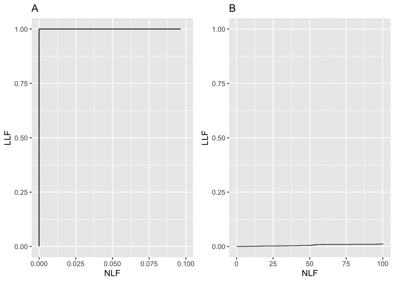
$A: raw FROC curve for $\mu=10$, B: raw FROC for $\mu=0.01$.$

FIGURE 24.4: A: raw FROC curve for $\mu=10$, B: raw FROC for $\mu=0.01$.

Fig. 24.4: (A): FROC plot for $\mu = 10$. Note the small range of the NLF axis (it only extends to 0.1). In this limit the ordinate reaches unity, but the abscissa is limited to a small value. (B): This plot corresponds to $\mu = 0.01$, depicting near chance-level performance. Note the greatly increased traverse in the x-directions and the slight upturn in the plot near $\text{NLF} = 100$.

The slope of the population FROC, assuming all suspicious regions are marked, decreases monotonically as the operating point moves up the curve, always staying non-negative, and it approaches zero, flattening out at an ordinate generally less than unity. LLF reaches unity for large $\mu$, which can be confirmed by setting $\mu$ to a large value, e.g., $\mu = 10$, as in Fig. 24.4 plot (A). [On the unit variance normal distribution scale, a value of 10, equivalent to 10 standard deviations, is effectively infinite.]

24.9 Perceptual SNR

Most readers, especially those with engineering backgrounds, are familiar with the concept of signal-to-noise-ratio, SNR. The shape and extent of the FROC plot is to a large extent determined by the perceptual¹⁸ SNR of the lesions, pSNR, modeled by the $\mu$ parameter. Perceptual SNR is the ratio of perceptual signal to perceptual noise. To get to perceptual variables one needs a model of the eye-brain system that transforms physical image brightness variations to corresponding perceived brightness variations, and such models exist (Van den Branden Lambrecht and Verscheure 1996; Daly 1993; Lubin 1995). For uniform background images, like the phantom images used by Bunch et al, physical signal can be measured by a template function that has the same attenuation profile as the true lesion. Assuming the template is aligned with the lesion the cross-correlation between the template function and the image pixel values is related to the numerator of SNR. The cross correlation is defined as the summed product of template function pixel values times the corresponding pixel values in the actual image. Next, one calculates the cross-correlation between the template function and the pixel values in the image when the template is centered over regions known to be lesion free. Subtracting the mean of these values (over several lesion free regions) from the centered value gives the numerator of SNR. The denominator is the standard deviation of the cross correlation values in the lesion free areas. Details on calculating physical SNR are in my CAMPI (computer analysis of mammography phantom images) work (Chakraborty, Sivarudrappa, and Roehrig 1999; Chakraborty and Fatouros 1998; D. P. Chakraborty 1997 a, 1997 b). To calculate perceptual SNR one repeats these measurements but the visual process, or some model of it (e.g., the Sarnoff JNDMetrix visual discrimination model (Lubin 1995; Siddiqui et al. 2005; Chakraborty 2006 a)), is used to filter the image prior to calculation of the cross-correlations.

An analogy may be helpful at this point. Finding the sun in the sky is a search task, so it can be used to illustrate important concepts.

24.10 The “solar” analogy: search vs. classification performance

Consider the sun, regarded as a “lesion” to be detected, with two daily observations spaced 12 hours apart, so that at least one observation period is bound to have the sun “somewhere up there”. Furthermore, the observer is assumed to know their GPS coordinates and have a watch that gives accurate local time, from which an accurate location of the sun can be deduced. Assuming clear skies and no obstructions to the view, the sun will always be correctly located and no reasonable observer will ever generate a non-lesion localization or NL, i.e., no region of the sky will be erroneously “marked”.

FROC curve implications of this analogy are:

Each 24-hour day corresponds to two “trials” in the (Egan, Greenburg, and Schulman 1961) sense, or two cases – one diseased and one non-diseased – in the medical imaging context.
The denominator for calculating LLF is the total number of AM days, and the denominator for calculating NLF is twice the total number of 24-hour days.
Most important, $\text{LLF}_{\text{max}} = 1$ and $\text{NLF}_{\text{max}} = 0$.

In fact, even when the sun is not directly visible due to heavy cloud cover, since the actual location of the sun can be deduced from the local time and GPS coordinates, the rational observer will still “mark” the correct location of the sun and not make any false sun localizations or “non-lesion localizations”, NLs. Consequently, even in this example $\text{LLF}_{\text{max}} = 1$ and $\text{NLF}_{\text{max}} = 0$.

The conclusion is that in a task where a target is known to be present in the field of view and its location is known, the observer will always reach $\text{LLF}_{\text{max}} = 1$ and $\text{NLF}_{\text{max}} = 0$. Why are LLF and NLF subscripted max? By randomly not marking the position of the sun even though it is visible, for example, using a coin toss to decide whether or not to mark the sun, the observer can “walk down” the y-axis of the FROC plot, reaching $LLF = 0$ and $NLF = 0$. Alternatively, the observer uses a very large threshold for reporting the sun, and as this threshold is lowered the operating point “walks down” the curve. The reason for allowing the observer to “walk down” the vertical is simply to demonstrate that a continuous FROC curve from the origin to the highest point (0,1) can, in fact, be realized.

Now consider a fictitious otherwise earth-like planet where the sun can be at random positions, rendering GPS coordinates and the local time useless. All one knows is that the sun is somewhere, in the upper or lower hemispheres subtended by the sky. If there are no clouds and consequently one can see the sun clearly during daytime, a reasonable observer would still correctly located the sun while not marking the sky with any incorrect sightings, so $\text{LLF}_{\text{max}} = 1$ and $\text{NLF}_{\text{max}} = 0$. This is because, in spite of the fact that the expected location is unknown, the high contrast sun is enough the trigger the peripheral vision system, so that even if the observer did not start out looking in the correct direction, peripheral vision will drag the observer’s gaze to the correct location for foveal viewing.

The implication of this is that fundamentally different mechanisms from that considered in conventional observer performance methodology, namely search and lesion-classification, are involved. Search describes the process of finding the lesion while not finding non-lesions. Once a possible sun location has been found, classification describes the process, of recognizing that it is indeed the sun and marking it. Recall that search involves two steps: finding the object of the search and acting on it. Search and lesion-classification performances describe the abilities of an observer to efficiently perform these steps.

Think of the eye as two cameras: a low-resolution camera (peripheral vision) with a wide field-of-view plus a high-resolution camera (foveal vision) with a narrow field-of-view If one were limited to viewing with the high-resolution camera one would spend so much time steering the high-resolution narrow field-of-view camera from spot-to-spot that one would have a hard time finding the desired stellar object. Having a single high-resolution narrow field of view vision would also have negative evolutionary consequences as one would spend so much time scanning and processing the surroundings with the narrow field of view vision that one would miss dangers or opportunities. Nature has equipped us with essentially two cameras; the first low-resolution camera is able to “digest” large areas of the surround and process it rapidly so that if danger (or opportunity) is sensed, then the eye-brain system rapidly steers the second high-resolution camera to the location of the danger (or opportunity). This is Nature’s way of optimally using the eye-brain system. For a similar reason astronomical telescopes come with a wide field of view lower resolution “spotter scope”.

Since the large field-of-view low-resolution peripheral vision system has complementary properties to the small field-of-view high-resolution foveal vision system, one expects an inverse correlation between search and lesion-classification performances. Stated generally, search involves two complementary processes: finding the suspicious regions and deciding if the found region is actually a lesion, and that there should be an inverse correlation between performance in the two tasks, see TBA Chapter 19.

When cloud cover completely blocks the fictitious random-position sun there is no stimulus to trigger the peripheral vision system to guide the fovea to the correct location. Lacking any stimulus, the observer is reduced to guessing and is led to different conclusions depending upon the benefits and costs involved. If, for example, the guessing observer earns a dollar for each LL and is fined a dollar for each NL, then the observer will likely not make any marks as the chance of winning a dollar is much smaller than losing many dollars. For this observer $\text{LLF}_{\text{max}} = 0$ and $\text{NLF}_{\text{max}} = 0$, and the operating point is “stuck” at the origin. If, on the other hand, the observer is told every LL is worth a dollar and there is no penalty to NLs, then with no risk of losing the observer will “fill up” the sky with marks. In either situation the locations of the marks will lie on a grid determined by the ratio of the $4\pi$ solid angle (subtended by the spherical sky) and the solid angle $\Omega$ subtended by the sun. By marking every possible grid location the observer is trivially guaranteed to “detect” the sun and earn a dollar irrespective of its random location and reach $LLF = 1$, but now the observer will generate lots of non-lesion localizations, so $\text{NLF}_{\text{max}}$ will be large:

\[\text{NLF}_{\text{max}} = 4\pi/\Omega\]

The FROC plot for this guessing observer is the straight line joining (0,0) to $(\text{NLF}_{\text{max}},1)$. For example, if the observer fills up half the sky then the operating point, averaged over many trials, is

\[(0.5 \times \text{NLF}_{\text{max}},0.5)\]

Radiologists do not guess – there is much riding on their decisions – so in the clinical situation, if the lesion is not seen, the radiologist will not mark the image at random.

The analogy is not restricted to the sun, which one might argue is an almost infinite SNR object and therefore atypical. As another example, consider finding stars or planets. In clear skies, if one knows the constellations, one can still locate bright stars and planets like Venus or Jupiter. With less bright stars and / or obscuring clouds, there will be false-sightings and the FROC plot could approach a flat horizontal line at ordinate equal to zero, but the observer will not fill up the sky with false sightings of a desired star.

False sightings of objects in astronomy do occur. Finding a new astronomical object is a search task, where as always one can have two outcomes, correct localization (LL) or incorrect localizations (NLs). At the time of writing there is a hunt for a new planet, possibly a gas giant , that is much further than even the newly demoted Pluto. There is an astronomer in Australia who is particularly good at finding super novae (an exploding star; one has to be looking in the right region of the sky at the right time to see the relatively brief explosion). His equipment is primitive by comparison to the huge telescope at Mt. Palomar, but his advantage is that he can rapidly point his 15" telescope at a new region of the sky and thereby cover a lot more sky, in a given unit of time, than is possible with the 200" Mt. Palomar telescope. His search expertise is particularly good. Once correctly pointed at the Mt. Palomar telescope will reveal a lot more detail about the object than is possible with the smaller telescope, i.e., the analogy is to high lesion-classification accuracy. In the medical imaging context this detail (the shape of the lesion, its edge characteristics, presence of other abnormal features, etc.) allows the radiologist to diagnose whether the lesion is malignant or benign. Once again one sees that there should be an inverse correlation between search and lesion-classification performances.

24.11 Discussion and suggestions

This chapter has introduced the FROC paradigm, the terminology used to describe it and a common operating characteristic associated with it, namely the FROC. There are several areas of possible confusion to avoid which consider the following suggestions:

Avoid using the term “lesion-specific” to describe location-specific paradigms.
Avoid using the term “lesion” when one means a “suspicious region” that may or may not be a true lesion.
Avoid using ROC-specific terms, such as true positive and false positive, that apply to the whole case, to describe location-specific terms such as lesion and non-lesion localization, that apply to localized regions of the image. This issue will come up in later chapters.
Avoid using the FROC-1 rating to mean in effect “I see no signs of disease in this image”, when in fact it should be used as the lowest level of a reportable suspicious region. The former usage amounts to wasting a confidence level.
Do not show FROC curves as reaching the unit ordinate, as this is the exception rather than the rule.
Do not conceptualize FROC curves as extending to large values to the right.
Arbitrariness of the proximity criterion and multiple marks in the same region are not clinically important. Interactions with clinicians will allow selection of an appropriate proximity criterion for the task at hand and the multiple mark problem only occurs with algorithmic observers and is readily fixed.

Additional points made in this chapter are: There is an inverse correlation between $\text{LLF}_{\text{max}}$ and $\text{NLF}_{\text{max}}$, analogous to that been sensitivity and specificity in ROC analysis. The observed end-point $(\text{NLF}_{\text{max}}, \text{LLF}_{\text{max}})$ of the FROC curve tends to approach the point (0,1) as the perceptual SNR of the lesions approaches infinity. The solar analogy is relevant to understanding the search task. In search tasks two types of expertise are at work: search and lesion-classification performances, and there exists an expected inverse correlation between them.

The FROC plot is the first proposed way of visually summarizing FROC data. The next chapter deals with all empirical operating characteristics that can be defined from an FROC dataset.

24.12 References

References

Alberdi, Eugenio, Andrey A Povyakalo, Lorenzo Strigini, Peter Ayton, and Rosalind Given-Wilson. 2008. “CAD in Mammography: Lesion-Level Versus Case-Level Analysis of the Effects of Prompts on Human Decisions.” International Journal of Computer Assisted Radiology and Surgery 3 (1-2): 115–22.

Black, William C. 2000. “Anatomic Extent of Disease: A Critical Variable in Reports of Diagnostic Accuracy.” Journal Article. Radiology 217 (2): 319–20. http://radiology.rsnajnls.org.

Black, William C., and Andrew J. Dwyer. 1990. “Local Versus Global Measures of Accuracy: An Important Distinction for Diagnostic Imaging.” Journal Article. Med Decis Making 10 (4): 266–73. https://doi.org/10.1177/0272989x9001000404.

Bunch, Philip C, John F Hamilton, Gary K Sanderson, and Arthur H Simmons. 1977. “A Free Response Approach to the Measurement and Characterization of Radiographic Observer Performance.” In Application of Optical Instrumentation in Medicine Vi, 127:124–35. International Society for Optics; Photonics.

Chakraborty, Dev P. 1989. “Maximum Likelihood Analysis of Free-Response Receiver Operating Characteristic (Froc) Data.” Medical Physics 16 (4): 561–68.

Chakraborty, Dev P. 2006a. “An Alternate Method for Using a Visual Discrimination Model (Vdm) to Optimize Softcopy Display Image Quality.” Journal Article. Journal of the Society for Information Display 14 (10): 921–26.

Chakraborty, Dev P., M. Sivarudrappa, and H. Roehrig. 1999. “Computerized Measurement of Mammographic Display Image Quality.” Conference Proceedings. In Proc Spie Medical Imaging 1999: Physics of Medical Imaging, edited by John M. Boone John M. Boone; James T. Dobbins III, 3659:131–41. SPIE.

Chakraborty, D. P. 1997a. “Comparison of Computer Analysis of Mammography Phantom Images (Campi) with Perceived Image Quality of Phantom Targets in the Acr Phantom.” Conference Proceedings. In Proc. SPIE Medical Imaging 1997: Image Perception, edited by Harold L. Kundel, 3036:160–67. SPIE.

Chakraborty, D. 1997b. “Computer Analysis of Mammography Phantom Images (Campi): An Application to the Measurement of Microcalcification Image Quality of Directly Acquired Digital Images.” Journal Article. Medical Physics 24 (8): 1269–77.

Chakraborty, D. P., E. S. Breatnach, M. V. Yester, B. Soto, G. T. Barnes, and R. G. Fraser. 1986. “Digital and Conventional Chest Imaging: A Modified ROC Study of Observer Performance Using Simulated Nodules.” Journal Article. Radiology 158: 35–39. https://doi.org/10.1148/radiology.158.1.3940394.

Chakraborty, D. P., and Panos P. Fatouros. 1998. “Application of Computer Analyis of Mammography Phantom Images (Campi) Methodology to the Comparison of Two Digital Biopsy Machines.” Conference Proceedings. In Proc Spie Medical Imaging 1998: Physics of Medical Imaging, edited by John M. Boone James T. Dobbins III, 3336:618–28. SPIE.

Daly, S. 1993. “The Visible Differences Predictor: An Algorithm for the Assessment of Image Fidelity.” Book Section. In Digital Images and Human Vision, edited by A. B. Watson, 179–206. Cambridge, Mass: MIT Press.

Dobbins III, James T, H Page McAdams, John M Sabol, Dev P Chakraborty, Ella A Kazerooni, Gautham P Reddy, Jenny Vikgren, and Magnus Båth. 2016. “Multi-Institutional Evaluation of Digital Tomosynthesis, Dual-Energy Radiography, and Conventional Chest Radiography for the Detection and Management of Pulmonary Nodules.” Journal Article. Radiology 282 (1): 236–50.

Egan, J. P., G. Z. Greenburg, and A. I. Schulman. 1961. “Operating Characteristics, Signal Detectability and the Method of Free Response.” Journal Article. J Acoust Soc. Am. 33: 993–1007.

Ernster, Virginia L. 1981. “The Epidemiology of Benign Breast Disease.” Journal Article. Epidemiologic Reviews 3 (1): 184–202.

Halpern, Scott D, Jason HT Karlawish, and Jesse A Berlin. 2002. “The Continuing Unethical Conduct of Underpowered Clinical Trials.” Journal Article. Jama 288 (3): 358–62.

Lubin, J. 1995. A Visual Discrimination Model for Imaging System Design and Evaluation. Book. Visual Models for Target Detection and Recognition. Singapore: World Scientific Publishers.

Miller, Harold. 1969. “The FROC Curve: A Representation of the Observer’s Performance for the Method of Free Response.” Journal Article. The Journal of the Acoustical Society of America 46 (6(2)): 1473–6.

Niklason, L. T., N. M. Hickey, Dev P. Chakraborty, E. A. Sabbagh, M. V. Yester, R. G. Fraser, and G. T. Barnes. 1986. “Simulated Pulmonary Nodules: Detection with Dual-Energy Digital Versus Conventional Radiography.” Journal Article. Radiology 160: 589–93. https://doi.org/10.1148/radiology.160.3.3526398.

Obuchowski, Nancy A., Michael L. Lieber, and Kimerly A. Powell. 2000. “Data Analysis for Detection and Localization of Multiple Abnormalities with Application to Mammography.” Journal Article. Acad. Radiol. 7 (7): 516–25.

Siddiqui, Khan M, Jeffrey P Johnson, Bruce I Reiner, and Eliot L Siegel. 2005. “Discrete Cosine Transform Jpeg Compression Vs. 2D Jpeg2000 Compression: JNDmetrix Visual Discrimination Model Image Quality Analysis.” In Medical Imaging 2005: PACS and Imaging Informatics, 5748:202–7. International Society for Optics; Photonics.

Starr, S. J., C. E. Metz, and L. B. Lusted. 1977. “Comments on Generalization of Receiver Operating Characteristic Analysis to Detection and Localization Tasks.” Journal Article. Phys. Med. Biol. 22: 376–79.

Swensson, Richard G. 1996. “Unified Measurement of Observer Performance in Detecting and Localizing Target Objects on Images.” Journal Article. Medical Physics 23 (10): 1709–25.

Van den Branden Lambrecht, Christian J, and Olivier Verscheure. 1996. “Perceptual Quality Measure Using a Spatiotemporal Model of the Human Visual System.” In Digital Video Compression: Algorithms and Technologies 1996, 2668:450–61. International Society for Optics; Photonics.

Diffuse interstitial lung disease refers to disease within both lungs that affects the interstitium or connective tissue that forms the support structure of the lungs’ air sacs or alveoli. When one inhales, the alveoli fill with air and pass oxygen to the blood stream. When one exhales, carbon dioxide passes from the blood into the alveoli and is expelled from the body. When interstitial disease is present, the interstitium becomes inflamed and stiff, preventing the alveoli from fully expanding. This limits both the delivery of oxygen to the blood stream and the removal of carbon dioxide from the body. As the disease progresses, the interstitium scars with thickening of the walls of the alveoli, which further hampers lung function.↩︎
When different views of the same patient anatomy (perhaps in different modalities) are available, it is assumed that all images are segmented consistently, and the rating for each ROI takes into account all views of that ROI in the different views (or modalities). The segmentation shown in the figure is a schematic. In fact the ROIs could be clinically driven descriptors of location, such as “apex of lung” or “mediastinum”, and the image does not have to have lines showing the ROIs (which would be distracting to the radiologist). The number of ROIs per image can be at the researcher’s discretion and there is no requirement that every case have a fixed number of ROIs.↩︎
The probability of benign suspicious regions is much higher (Ernster 1981), about 13% for women aged 40-45.↩︎
The proper terminology for this paradigm has evolved. Older publications and some newer ones refer to this as a true positive (TP) event, thereby confusing a ROC related term that does not involve search with one that does.↩︎
Generally the proximity criterion is more stringent for smaller lesions than for larger one. However, for very small lesions allowance is made so that the criterion does not penalize the radiologist for normal marking “jitter”. For 3D images the proximity criteria is different in the x-y plane vs. the slice thickness axis.↩︎
The exception would be if the perceived lesions were speck-like objects in a mammogram, and even here radiologists tend to broadly outline the region containing perceived specks – they do not mark individual specks with great precision.↩︎
The reason for using the highest rating is that this gives full and deserved credit for the localization. Other marks in the same vicinity with lower ratings need to be discarded from the analysis; specifically, they should not be classified as NLs, because each mark has successfully located the true lesion to within the clinically acceptable criterion, i.e., any one of them is a good decision because it would result in a patient recall and point further diagnostics to the true location.↩︎
Bunch et al actually used the terms “true positive” and “false positive” to describe these events. This practice, still used in publications in this field, is confusing because there is ambiguity about whether these terms, commonly used in the ROC paradigm, are being applied to the case as a whole or to specific regions in the case.↩︎
Fig. 5 in (Philip C Bunch et al. 1977) is incorrect in implying, with the arrows, that the plots extend indefinitely to the right. Also there is a notation differences: P(TP) in Bunch et. al. is equivalent to LLF in this book. To avoid confusion with the $\lambda$ parameter of the radiological search model, the variable Bunch et al. call $\lambda$ is equivalent to NLF in this book.↩︎
Since humans make the decisions, it would be incorrect to label these as physical signal-to-noise-ratios; that is the reason for qualifying them as perceptual SNRs.↩︎