Chapter 9 RSM fitting
9.2 TBA Introduction
Early work, reported in my 2017 print book, revealed that an FROC curve based estimation method worked only for designer level CAD data and not for human observer data. Subsequent effort focused on ROC curve-based fitting, and this proved successful at fitting radiologist datasets where detailed definition of the ROC curve is not available. A preliminary account of this work can be found in a conference proceeding (DP Chakraborty and Svahn 2011).
The reader should be surprised to learn that the ROC curve based fitting works, which implies that one does not even need FROC data to estimate RSM parameters. I have previously stated that the ROC paradigm ignores search, so how can one estimate search-model parameters from ROC data? The reason is that the shape of the RSM-predicted ROC curve and the location of the end-point depend on the RSM parameters.
9.3 ROC Likelihood function
In Chapter 6 expressions were derived for the coordinates \((x,y)\) of the ROC curve predicted by the RSM, see Eqn. (6.11) and Eqn. (6.15), where \(x\equiv x(\zeta,\lambda)\) and \(y \equiv y(\zeta , \mu, \lambda, \nu, \overrightarrow{f_L})\). Let \((F_r,T_r)\) denote the number of false positives and true positives in ROC rating bin \(r\) defined by thresholds \([\zeta_r, \zeta_{r+1})\), for \(r = 0, 1, ..., R_{FROC}\). \((F_0,T_0)\) represent the known numbers of non-diseased and diseased cases, respectively, with no marks, \((F_1,T_1)\) represent the corresponding numbers with highest rating equal to one, etc.
The probability \(P_{1r}\) of a count in non-diseased ROC bin \(r\) is:
\[\begin{equation} P_{1r} = x\left ( \zeta_r \right ) - x\left ( \zeta_{r+1} \right )\\ \tag{9.1} \end{equation}\]
The probability \(P_{2r}\) of a count in diseased ROC bin \(r\) is:
\[\begin{equation} P_{2r} = y\left ( \zeta_r \right ) - y\left ( \zeta_{r+1} \right )\\ \tag{9.2} \end{equation}\]
Ignoring combinatorial factors that do not depend on parameters the likelihood function is:
\[\left ( P_{1r} \right )^{F_r} \left ( P_{2r} \right )^{T_r}\]
The log-likelihood function is:
\[\begin{equation} LL_{ROC} \left ( \mu, \lambda, \nu, \overrightarrow{f_L} \right )= \sum_{r=0}^{R_{FROC}} \left [F_r log \left (P_{1r} \right ) + T_r log \left (P_{2r} \right ) \right ] \\ \tag{9.3} \end{equation}\]
The total number of parameters to be estimated, including the \(R_{FROC}\) thresholds, is \(3+R_{FROC}\). Maximizing the likelihood function yields estimates of the RSM parameters.
The Broyden–Fletcher–Goldfarb–Shanno (BFGS) (Shanno and Kettler 1970; Shanno 1970; Goldfarb 1970; Fletcher 1970, 2013; Broyden 1970) minimization algorithm, as implemented as function mle2() in R-package bbmle (Bolker and R Development Core Team 2022) was used to minimize the negative of the likelihood function. Since the BFGS-algorithm varies each parameter in an unrestricted range \((-\infty, \infty)\), which would cause problems (e.g., RSM physical parameters cannot be negative and thresholds need to be properly ordered), appropriate variable transformations (both “forward” and “inverse”) were used so that parameters supplied to the log-likelihood function were always in the valid range, irrespective of values chosen by the BFGS-algorithm.
9.4 Implementation
Function FitRsmROC() fits an RSM-predicted ROC curve to a binned single-modality single-reader ROC dataset. It is called by ret <- FitRsmRoc(binnedRocData, lesDistr, trt = 1, rdr = 1), where binnedRocData is a binned multi-treatment multi-reader ROC dataset, lesDistr is the lesion distribution vector for the dataset and trt and rdr are the desired treatment and reader to extract from the dataset, each of which defaults to one.
The return value ret is a list with the following elements:
ret$muThe RSM \(\mu\) parameter.ret$lambdaThe RSM \(\lambda\) parameter.ret$nuThe RSM \(\nu\) parameter.ret$zetasThe RSM \(\zeta\) parameters.ret$AUCThe RSM fitted ROC-AUC.ret$StdAUCThe standard deviation of AUC.ret$NLLIniThe initial value of negative log-likelihood.ret$NLLFinThe final value of negative log-likelihood.ret$ChisqrFitStatsThe chisquare goodness of fit (if it can be calculated).ret$covMatThe covariance matrix of the parameters (if it can be calculated).ret$fittedPlotAggplotobject containing the fitted plots along with the empirical operating points and error bars.
9.5 FitRsmROC usage example
- The following example uses the first treatment in
dataset04; this is a 5 treatment 4 radiologist FROC dataset (Federica Zanca et al. 2009) consisting of 200 cases acquired on a 5-point integer scale, i.e., it is already binned. If not one needs to bin the dataset usingDfBDataset(). The number of parameters to be estimated increases with the number of bins: for each additional bin one needs to estimate an additional cutoff parameter.
rocData <- DfFroc2Roc(dataset04)
lesDistr <- UtilLesionDistrVector(dataset04)
ret <- FitRsmRoc(rocData, lesDistr = lesDistr)
The lesion distribution vector is 0.69, 0.2, 0.11. This means that fraction 0.69 of each diseased case contains one lesion, fraction 0.2 contains two lesions and fraction 0.11 contains three lesions. Since the fitted curve depends on the lesion distribution the fitting function needs to know this distribution. 31
The fitted parameter values are as follows (all cutoffs excepting \(\zeta_1\), the chi-square statistic and the covariance matrix, are not shown):
- \(\mu\) = 3.658
- \(\lambda\) = 9.935
- \(\nu\) = 0.796
- \(\zeta_1\) = 1.504
- \(\text{AUC}\) = 0.9064
- \(\sigma (\text{AUC})\) = 0.023
- \(\text{NLLIni}\) = 281.4
- \(\text{NLLFin}\) = 267.27
The relatively large separation parameter \(\mu\) implies good lesion-classification performance. The large \(\lambda\) parameter implies poor lesion-localization performance. On the average the observer generates 9.94 latent NL marks per image. However, because of the relatively large value of \(\zeta_1\), i.e., 1.5, only fraction 0.066 of these are actually marked, resulting in 0.66 actual marks per image. Lesion-localization performance depends on the numbers of latent marks, i.e., \(\lambda\) and \(\nu\), not the actual numbers of marks.
The fitting program decreased the negative of the log-likelihood function from 281.4 to 267.27. A decrease in negative log-likelihood is equivalent to an increase in the likelihood, which is as expected, as the function maximizes the log-likelihood.
Because the RSM contains 3 parameters, which is one more than conventional ROC models, the chisquare goodness of fit statistic usually cannot be calculated, except for large datasets - the criterion of 5 counts in each bin for true positives and false positives is usually hard to meet. Using the method described in RJafrocRocBook the degrees of freedom is \(\text{df} = R_{FROC} - 3\).32
Shown next is the fitted plot. Error bars (exact 95% confidence intervals) are shown for the lowest and highest operating points.
print(ret$fittedPlot)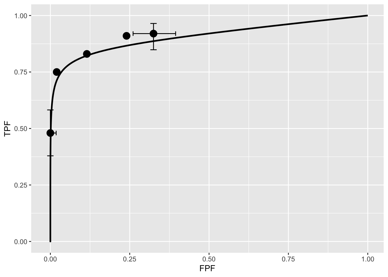
The fitted ROC curve is proper: it’s slope decreases monotonically as one moves up the curve thereby ruling out hooks such as are predicted by the binormal model. The area under the proper ROC (calculated by numerical integration of the RSM-predicted curve) is 0.906 which will be shown in a subsequent chapter TBA to be identical to that yielded by other proper ROC fitting methods and higher than the binormal model fitted value.
9.6 Discussion / Summary
Over the years, there have been several attempts at fitting FROC data. Prior to the RSM-based ROC curve approach described in this chapter, all methods were aimed at fitting FROC curves in the mistaken belief that this approach was using all the data. The earliest was my FROCFIT software (Dev P. Chakraborty 1989). This was followed by Swensson’s approach (Swensson 1996), subsequently shown to be equivalent to my earlier work, as far as predicting the FROC curve was concerned (DP Chakraborty and Yoon 2008). In the meantime, CAD developers, who relied heavily on the FROC curve to evaluate their algorithms, developed an empirical approach that was subsequently put on a formal basis in the IDCA (initial detection and candidate analysis) method (Edwards et al. 2002). While this method works with CAD data it fails with radiologist data – the reason is that it assumes \(\zeta_1 = -\infty\) which is not true for radiologists (this is discussed in my 2017 print book).
This chapter describes an approach to fitting ROC curves using the RSM. On the face of it fitting the ROC curve seems to be ignoring much of the data. For example the ROC rating on a non-diseased case is the rating of the highest-rated mark on that image, or negative infinity if the case has no marks. If the case has several NL marks, only the highest rated one is used. In fact the highest rated mark contains information about the other marks on the case, namely they were all rated lower. The statistical term for this is sufficiency (Larsen and Marx 2005). As an example, the highest of a number of samples from a uniform distribution is a sufficient statistic, i.e., it contains all the information contained in the observed samples. While not quite the same for normally distributed values, neglect of the NLs rated lower is not as bad as might seem at first.
The next chapter describes application of the RSM and other available proper ROC fitting methods to a number of datasets.