Chapter 10 F-distribution
10.2 Background
A number of vignettes used to be part of the RJafroc package. These have been moved here.
10.3 Introduction
Since it plays an important role in sample size estimation, it is helpful to examine the behavior of the F-distribution. In the following ndf = numerator degrees of freedom, ddf = denominator degrees of freedom and ncp = non-centrality parameter (i.e., the \(\Delta\) appearing in Eqn. (11.6) of (Dev P. Chakraborty 2017)).
The use of three R functions is demonstrated.
qf(p,ndf,ddf)is the quantile function of the F-distribution for specified values ofp,ndfandddf, i.e., the valuexsuch that fractionpof the area under the F-distribution lies to the right ofx. Sincencpis not included as a parameter, the default value, i.e., zero, is used. This is called the central F-distribution.df(x,ndf,ddf,ncp)is the probability density function (pdf) of the F-distribution, as a function ofx, for specified values ofndf,ddfandncp.pf(x,ndf,ddf,ncp)is the probability (or cumulative) distribution function of the F-distribution for specified values ofndf,ddfandncp.
10.4 Effect of ncp for ndf = 2 and ddf = 10
- Four values of
ncpare considered (0, 2, 5, 10) forddf= 10. fCritis the critical value of the F distribution, i.e., that value such that fraction \(\alpha\) of the area is to the right of the critical value, i.e.,fCritis identical in statistical notation to \({{F}_{1-\alpha ,ndf,ddf}}\).
ndf <- 2;ddf <- 10;ncp <- c(0,2,5,10)
alpha <- 0.05
fCrit <- qf(1-alpha, ndf,ddf)
x <- seq(1, 20, 0.1)
myLabel <- c("A", "B", "C", "D")
myLabelIndx <- 1
pFgtFCrit <- NULL
for (i in 1:length(ncp))
{
  y <- df(x,ndf,ddf,ncp=ncp[i])
  pFgtFCrit <- c(pFgtFCrit, 1-pf(fCrit, ndf, ddf, ncp = ncp[i]))
}
for (i in 1:length(ncp))
{
  y <- df(x,ndf,ddf,ncp=ncp[i])
  curveData <- data.frame(x = x, pdf = y)
  curvePlot <- ggplot(data = curveData, mapping = aes(x = x, y = pdf)) +
    geom_line() +
    ggtitle(myLabel[myLabelIndx]);myLabelIndx <- myLabelIndx + 1
  print(curvePlot)
}
fCrit_2_10 <- fCrit # convention fCrit_ndf_ddf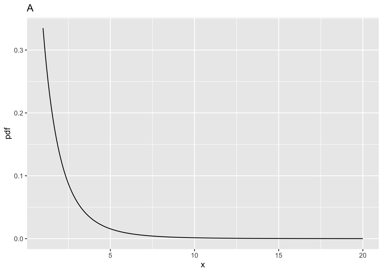
| ndf | ddf | fCrit | ncp | pFgtFCrit | |
|---|---|---|---|---|---|
| A | 2 | 10 | 4.102821 | 0 | 0.0500000 |
| B | 2 | 10 | 4.102821 | 2 | 0.1775840 |
| C | 2 | 10 | 4.102821 | 5 | 0.3876841 |
| D | 2 | 10 | 4.102821 | 10 | 0.6769776 |
10.6 Effect of ncp for ndf = 2 and ddf = 100
| ndf | ddf | fCrit | ncp | pFgtFCrit | |
|---|---|---|---|---|---|
| A | 2 | 10 | 4.102821 | 0 | 0.0500000 |
| B | 2 | 10 | 4.102821 | 2 | 0.1775840 |
| C | 2 | 10 | 4.102821 | 5 | 0.3876841 |
| D | 2 | 10 | 4.102821 | 10 | 0.6769776 |
| E | 2 | 100 | 3.087296 | 0 | 0.0500000 |
| F | 2 | 100 | 3.087296 | 2 | 0.2199264 |
| G | 2 | 100 | 3.087296 | 5 | 0.4910802 |
| H | 2 | 100 | 3.087296 | 10 | 0.8029764 |
10.7 Comments
- All comparisons in this sections are at the same values of
ncpdefined above. - And between
ddf= 100 andddf= 10.
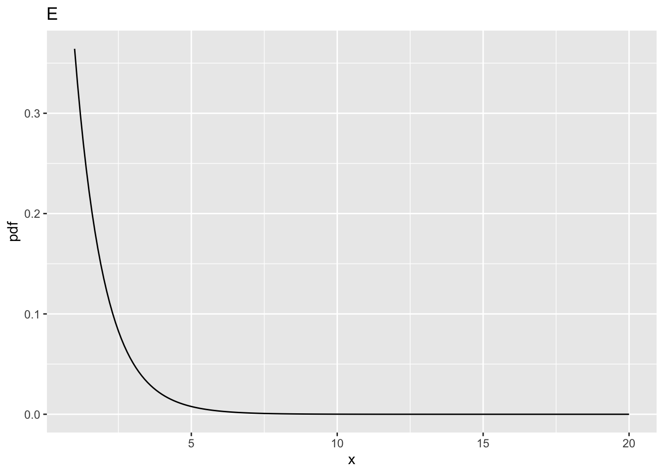
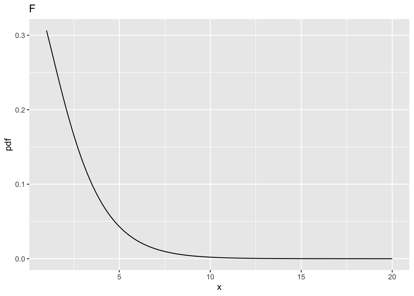
10.7.1 Fig. E
- This corresponds to
ncp= 0,ndf= 2 andddf= 100. - The critical value is
fCrit_2_100= 3.0872959. Notice the decrease compared to the previous value forncp= 0, i.e., 4.102821, forddf= 10. - One expects that increasing
ddfwill make it more likely that the NH will be rejected, and this is confirmed below. - All else equal, statistical power increases with increasing
ddf.
10.7.2 Fig. F
- This corresponds to
ncp= 2,ndf= 2 andddf= 100. - The probability of exceeding the critical value is
prob > fCrit_2_100= 0.2199264, greater than the previous value, i.e., 0.177584 forddf= 10.
10.8 Effect of ncp for ndf = 1, ddf = 100
| ndf | ddf | fCrit | ncp | pFgtFCrit | |
|---|---|---|---|---|---|
| A | 2 | 10 | 4.102821 | 0 | 0.0500000 |
| B | 2 | 10 | 4.102821 | 2 | 0.1775840 |
| C | 2 | 10 | 4.102821 | 5 | 0.3876841 |
| D | 2 | 10 | 4.102821 | 10 | 0.6769776 |
| E | 2 | 100 | 3.087296 | 0 | 0.0500000 |
| F | 2 | 100 | 3.087296 | 2 | 0.2199264 |
| G | 2 | 100 | 3.087296 | 5 | 0.4910802 |
| H | 2 | 100 | 3.087296 | 10 | 0.8029764 |
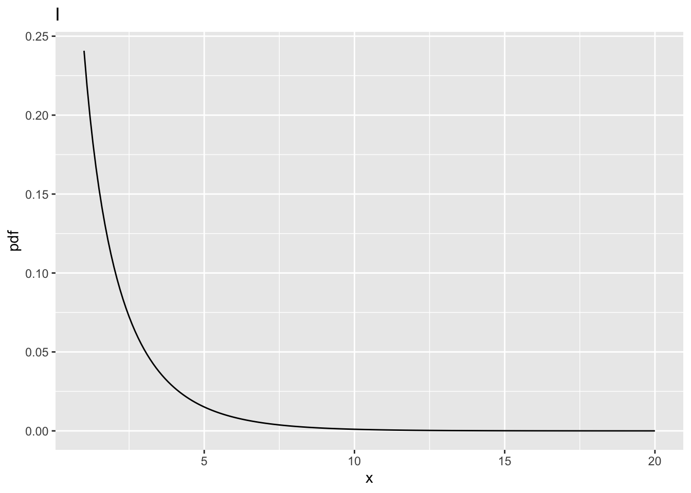
| I | 1 | 100 | 3.936143 | 0 | 0.0500000 |
| J | 1 | 100 | 3.936143 | 2 | 0.2883607 |
| K | 1 | 100 | 3.936143 | 5 | 0.6004962 |
| L | 1 | 100 | 3.936143 | 10 | 0.8793619 |
10.9 Comments
- All comparisons in this sections are at the same values of
ncpdefined above and atddf= 100. - And between
ndf= 1 andndf= 2.
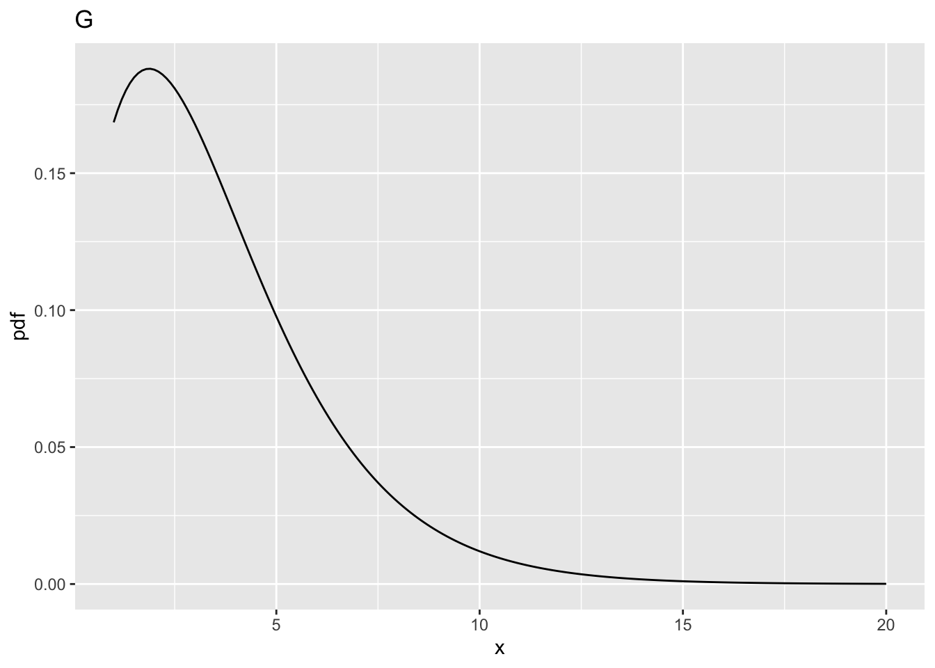
10.9.1 Fig. I
- This corresponds to
ncp= 0,ndf= 1 andddf= 100. - The critical value is
fCrit_1_100= 3.936143. - Notice the increase in the critical value as compared to the corresponding value for
ndf = 2, i.e., 3.0872959. - One expects power to decrease: the following code demonstrates that as
ndfincreases, the critical valuefCritdecreases. - In significance testing generally
ndf= I -1. - It more likely that the NH will be rejected with increasing numbers of treatments.
| ndf | ddf | fCrit |
|---|---|---|
| 1 | 100 | 3.936143 |
| 2 | 100 | 3.087296 |
| 5 | 100 | 2.305318 |
| 10 | 100 | 1.926692 |
| 12 | 100 | 1.850255 |
| 15 | 100 | 1.767530 |
| 20 | 100 | 1.676434 |
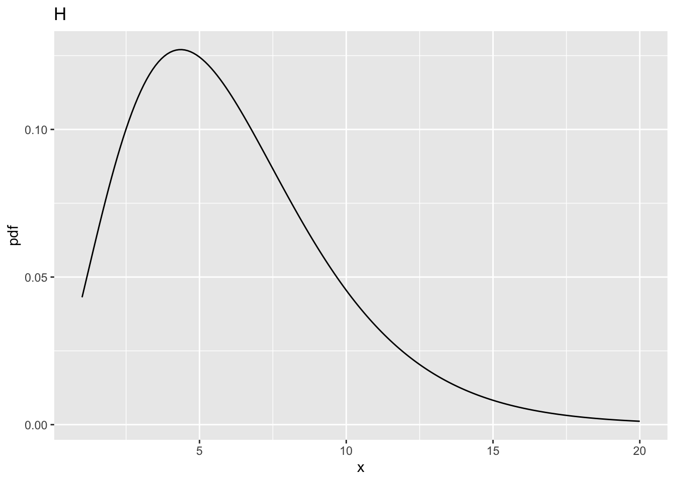
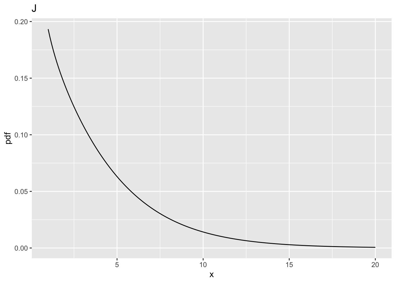
10.9.2 Fig. J
- This corresponds to
ncp= 2,ndf= 1 andddf= 100. - Now
prob > fCrit_1_100= 0.2883607, 0.1351602, 0.0168844, 8.9992114^{-4}, 3.2584757^{-4}, 8.1619807^{-5}, 1.1084132^{-5}, larger than the previous value 0.2199264. - The power has actually increased.
10.10 Summary
- Power increases with increasing
ddfandncp. - The effect of increasing
ncpis quite dramatic. This is because power depends on the square ofncp. - As
ndfincreases,fCritdecreases, which makes it more likely that the NH will be rejected. - With increasing numbers of treatments the probability is greater that the F-statistic will be large enough to exceed the critical value.
10.5 Comments
10.5.1 Fig. A
ncp = 0, i.e., the central F-distribution.fCritin the above code block, is the value ofxsuch that the probability of exceedingxis \(\alpha\). The corresponding parameteralphais defined above as 0.05.fCrit= 4.102821. Notice the use of the quantile functionqf()to determine this value, and the default value ofncp, namely zero, is used; specifically, one does not pass a 4th argument toqf().fCrit. As expected,prob > fCrit= 0.05 because this is howfCritwas defined.10.5.2 Fig. B
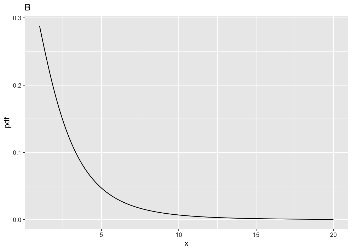
ncp = 2,ndf= 2 andddf= 10.prob > fCrit= 0.177584, i.e., the statistical power (compare this to Fig. A whereprob > fCritwas 0.05).10.5.3 Fig. C
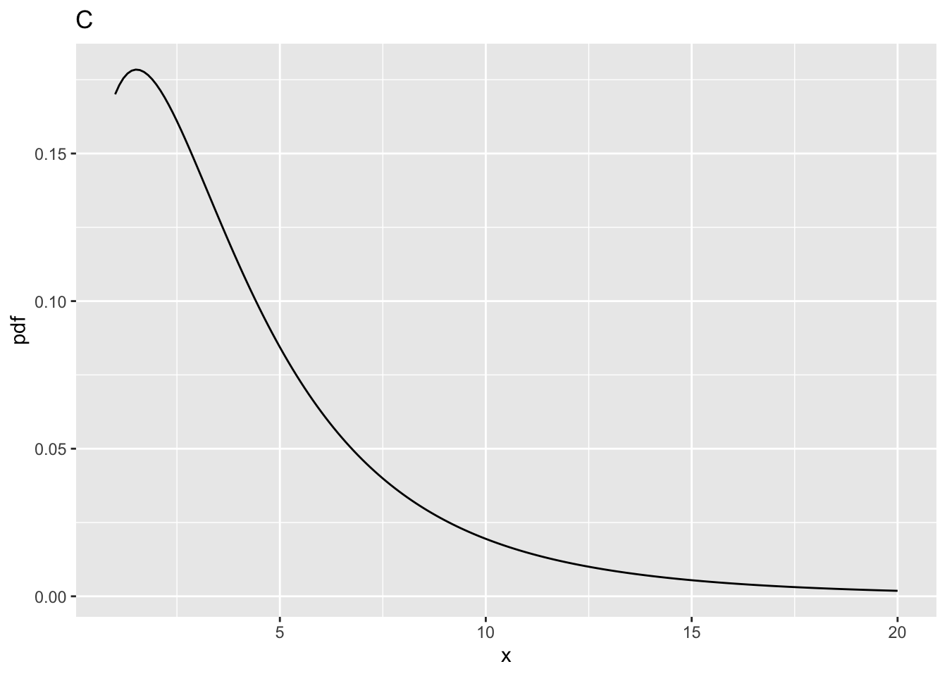
ncp = 5,ndf= 2 andddf= 10.prob > fCrit= 0.3876841.10.5.4 Fig. D
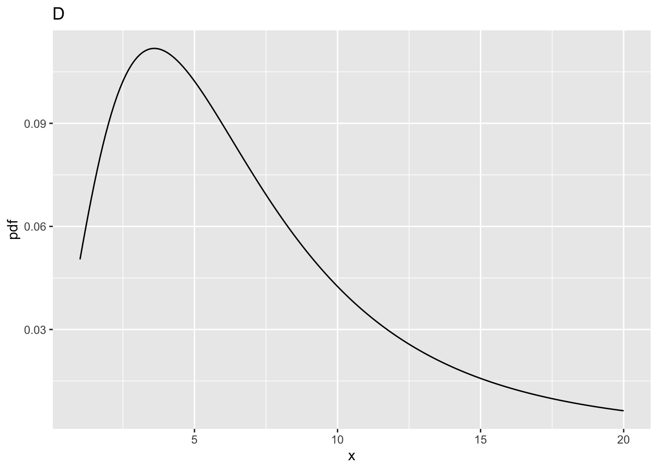
ncp = 10,ndf= 2 andddf= 10.prob > fCritis 0.6769776.x= 4.102821, fraction 0.6769776 of the probability distribution in Fig. D lies to the right of this line10.5.5 Summary
The larger that non-centrality parameter, the greater the shift to the right of the F-distribution, and the greater the statistical power.