Chapter 11 RSM operating characteristics
11.2 Introduction
- The purpose of this vignette is to explain the operating characteristics predicted by the RSM. It relates to Chapter 17 in my book (Dev P. Chakraborty 2017).
- This vignette is under development …
- Also to explain the difference between
datasetmembers (lesionID,lesionWeight) and RSM parameters (lesDistr,lesWghtDistr).
11.3 The distinction between predicted curves and empirical curves
- Operating characteristics predicted by a model have zero sampling variability.
- Empirical operating characteristics, which apply to datasets, have non-zero sampling variability.
- If the model is correct, as the numbers of cases in the dataset increases, the empirical operating characteristic asymptotically approaches the predicted curve.
11.4 The RSM model
- The 3 RSM parameters and two additional parameters characterizing the dataset determine the wAFROC curve.
- The 3 RSM parameters are \(\mu\), \(\lambda\) and \(\nu\).
- The two dataset parameters are:
- The distribution of number of lesions per diseased case,
lesDistr. - The distribution of lesion weights,
lesWghtDistr.
- The distribution of number of lesions per diseased case,
- These parameters do not apply to individual cases; rather they refer to a large population (asymptotically infinite in size) of cases.
str(dataset04$lesions$IDs)
#>  num [1:100, 1:3] 1 1 1 1 1 1 1 1 1 1 ...
str(dataset04$lesions$weights)
#> num [1:100, 1:3] 1 1 1 1 1 1 1 1 1 1 ...- Note that the first index of both arrays is the case index for the 100 abnormal cases in this dataset.
- With finite number of cases the empirical operating characteristic (or for that matter any fitted operating characteristic) will have sampling variability as in the following example.
11.5 The empirical wAFROC
p <- PlotEmpiricalOperatingCharacteristics(dataset04, opChType = "wAFROC")
p$Plot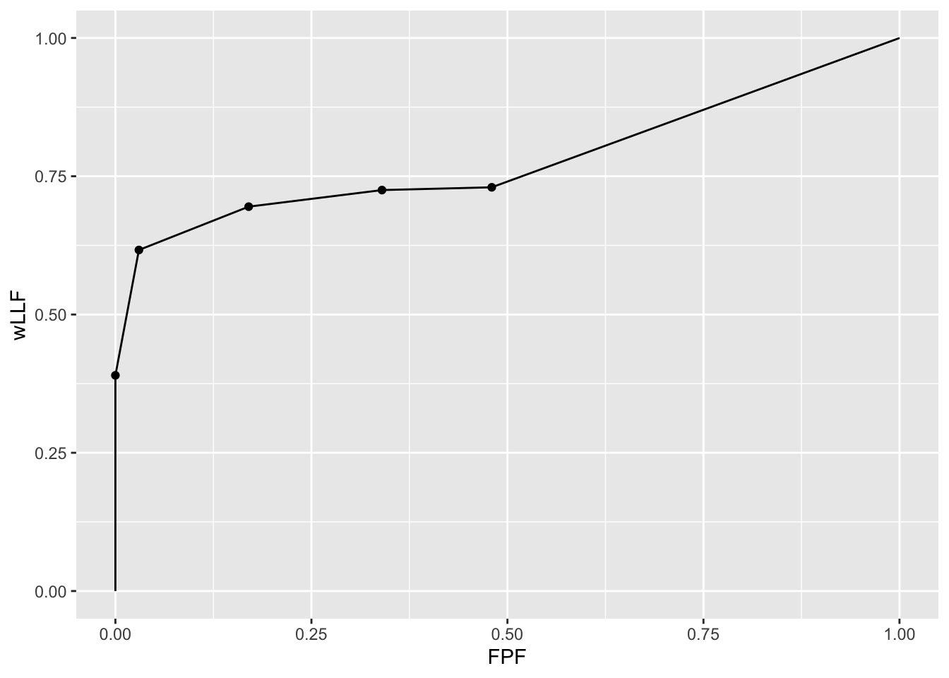
- The piecewise linear nature of the plot, with sharp breaks, indicates that this is due to a finite dataset.
- In contrast the following code shows a smooth plot, because it is a model predicted plot.
11.6 The predicted wAFROC
## Following example is for mu = 2, lambda = 1, nu = 0.6. 20% of the diseased
## cases have a single lesion, 40% have two lesions, 10% have 3 lesions,
## and 30% have 4 lesions.
lesDistr <- c(0.2, 0.4, 0.1, 0.3)

## On cases with one lesion the weights are 1, on cases with 2 lesions the weights
## are 0.4 and 0.6, on cases with three lesions the weights are 0.2, 0.3 and 0.5, and
## on cases with 4 lesions the weights are 0.3, 0.4, 0.2 and 0.1:
relWeights <- c(0.3,  0.4, 0.2,  0.1)
p <- PlotRsmOperatingCharacteristics(
  mu = 2,
  lambda = 1,
  nu = 0.6,
  OpChType = "wAFROC",
  lesDistr = lesDistr,
  relWeights = relWeights,
  legendPosition = "bottom", nlfRange = c(0, 1), llfRange = c(0, 1))
p$wAFROCPlot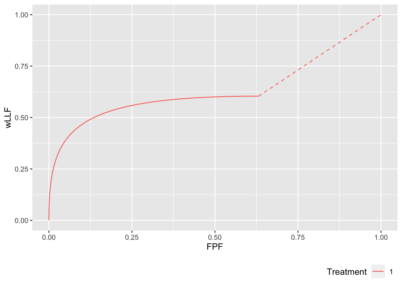
11.7 The distribution of number of lesions and weights
lesDistr
#> [1] 0.2 0.4 0.1 0.3
relWeights
#> [1] 0.3 0.4 0.2 0.1- The
lesDistrarray 0.2, 0.4, 0.1, 0.3 specifies the fraction of diseased cases with the number of lesions corresponding to the column index. To specify a dataset with exactly 3 lesions per diseased case uselesDist = c(0, 0, 1, 0). - The
relWeightsarray 0.3, 0.4, 0.2, 0.1 specifies the relative weights. - For cases with 1 lesion, the weight is 1.
- For cases with 2 lesions, the first lesion has weight 0.4285714 and the second lesion has weight 0.5714286, which are in the ratio 0.3 : 0.4 and sum to unity.
- For cases with 3 lesions, the first lesion has weight 0.3333333, the second lesion has weight 0.4444444 and the third lesion has weight 0.2222222, which are in the ratio 0.3 : 0.4 : 0.2, and sum to unity.
- For cases with 4 lesions, the weights are 0.3, 0.4, 0.2 and 0.1, which are in the ratio 0.3 : 0.4 : 0.2 : 0.1 and sum to unity.
11.8 Other operating characteristics
- By changing
OpChTypeone can generate other operating characteristics. - Note that lesiion weights argument is not needed for ROC curves. It is only needed for
wAFROCandwAFROC1curves.
lesDistr <- c(0.2, 0.4, 0.1, 0.3)
p <- PlotRsmOperatingCharacteristics(
  mu = 2,
  lambda = 1,
  nu = 0.6,
  OpChType = "ROC",
  lesDistr = lesDistr,
  legendPosition = "bottom")
p$ROCPlot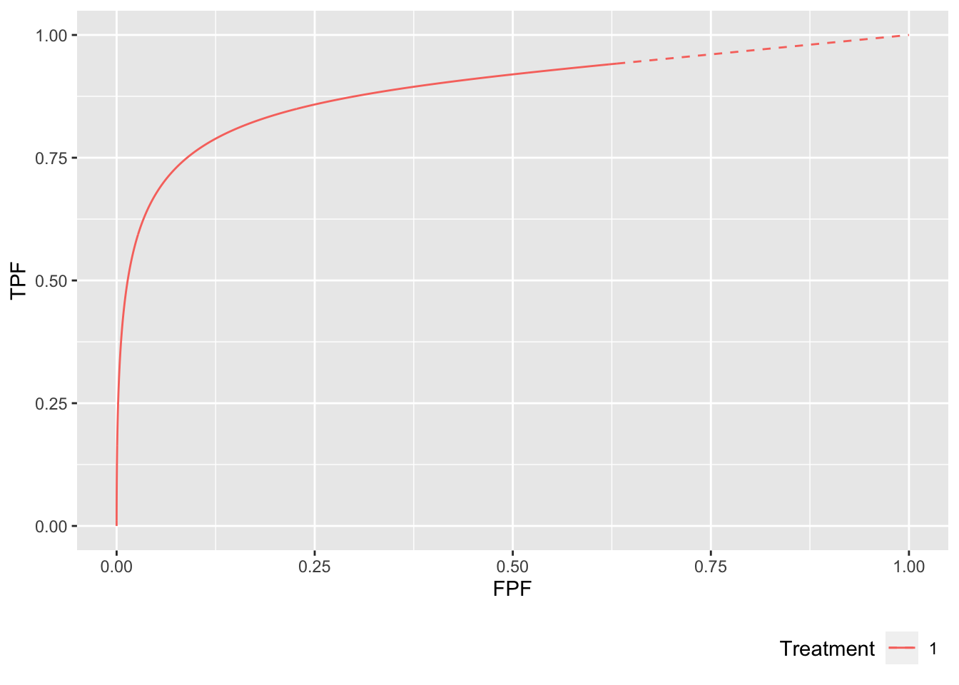
References
Chakraborty, Dev P. 2017. Observer Performance Methods for Diagnostic Imaging: Foundations, Modeling, and Applications with r-Based Examples. Boca Raton, FL: CRC Press.